MODFLOW 6 Tutorial 1: Unconfined Steady-State Flow Model

This tutorial demonstrates use of FloPy to develop a simple MODFLOW 6 model.

Getting Started

import os
import numpy as np
import matplotlib.pyplot as plt
import flopy

We are creating a square model with a specified head equal to h1 along all boundaries. The head at the cell in the center in the top layer is fixed to h2. First, set the name of the model and the parameters of the model: the number of layers Nlay, the number of rows and columns N, lengths of the sides of the model L, aquifer thickness H, hydraulic conductivity k

name = "tutorial01_mf6"
h1 = 100
h2 = 90
Nlay = 10
N = 101
L = 400.0
H = 50.0
k = 1.0

Create the Flopy Model Objects

One big difference between MODFLOW 6 and previous MODFLOW versions is that MODFLOW 6 is based on the concept of a simulation. A simulation consists of the following:

• Temporal discretization (TDIS)
• One or more models
• Zero or more exchanges (instructions for how models are coupled)
• Solutions

For this simple example, the simulation consists of the temporal discretization (TDIS) package, a groundwater flow (GWF) model, and an iterative model solution (IMS), which controls how the GWF model is solved.

Create the Flopy simulation object

sim = flopy.mf6.MFSimulation(
    sim_name=name, exe_name="mf6", version="mf6", sim_ws="."
)

Create the Flopy TDIS object

tdis = flopy.mf6.ModflowTdis(
    sim, pname="tdis", time_units="DAYS", nper=1, perioddata=[(1.0, 1, 1.0)]
)

Create the Flopy IMS Package object

ims = flopy.mf6.ModflowIms(sim, pname="ims", complexity="SIMPLE")

Create the Flopy groundwater flow (gwf) model object

model_nam_file = "{}.nam".format(name)
gwf = flopy.mf6.ModflowGwf(sim, modelname=name, model_nam_file=model_nam_file)

Now that the overall simulation is set up, we can focus on building the groundwater flow model. The groundwater flow model will be built by adding packages to it that describe the model characteristics.

Create the discretization (DIS) Package

Define the discretization of the model. All layers are given equal thickness. The bot array is build from H and the Nlay values to indicate top and bottom of each layer, and delrow and delcol are computed from model size L and number of cells N. Once these are all computed, the Discretization file is built.

bot = np.linspace(-H / Nlay, -H, Nlay)
delrow = delcol = L / (N - 1)
dis = flopy.mf6.ModflowGwfdis(
    gwf,
    nlay=Nlay,
    nrow=N,
    ncol=N,
    delr=delrow,
    delc=delcol,
    top=0.0,
    botm=bot,
)

Create the initial conditions (IC) Package

start = h1 * np.ones((Nlay, N, N))
ic = flopy.mf6.ModflowGwfic(gwf, pname="ic", strt=start)

Create the node property flow (NPF) Package

npf = flopy.mf6.ModflowGwfnpf(gwf, icelltype=1, k=k, save_flows=True)

Create the constant head (CHD) Package

List information is created a bit differently for MODFLOW 6 than for other MODFLOW versions. The cellid (layer, row, column, for a regular grid) can be entered as a tuple as the first entry. Remember that these must be zero-based indices!

chd_rec = []
chd_rec.append(((0, int(N / 4), int(N / 4)), h2))
for layer in range(0, Nlay):
    for row_col in range(0, N):
        chd_rec.append(((layer, row_col, 0), h1))
        chd_rec.append(((layer, row_col, N - 1), h1))
        if row_col != 0 and row_col != N - 1:
            chd_rec.append(((layer, 0, row_col), h1))
            chd_rec.append(((layer, N - 1, row_col), h1))
chd = flopy.mf6.ModflowGwfchd(
    gwf,
    maxbound=len(chd_rec),
    stress_period_data=chd_rec,
    save_flows=True,
)

The CHD Package stored the constant heads in a structured array, also called a numpy.recarray. We can get a pointer to the recarray for the first stress period (iper = 0) as follows.

iper = 0
ra = chd.stress_period_data.get_data(key=iper)
ra

rec.array([((0, 25, 25),  90.), ((0, 0, 0), 100.), ((0, 0, 100), 100.),
           ..., ((9, 100, 99), 100.), ((9, 100, 0), 100.),
           ((9, 100, 100), 100.)],
          dtype=[('cellid', 'O'), ('head', '<f8')])

# Create the output control (`OC`) Package
headfile = "{}.hds".format(name)
head_filerecord = [headfile]
budgetfile = "{}.cbb".format(name)
budget_filerecord = [budgetfile]
saverecord = [("HEAD", "ALL"), ("BUDGET", "ALL")]
printrecord = [("HEAD", "LAST")]
oc = flopy.mf6.ModflowGwfoc(
    gwf,
    saverecord=saverecord,
    head_filerecord=head_filerecord,
    budget_filerecord=budget_filerecord,
    printrecord=printrecord,
)

Create the MODFLOW 6 Input Files and Run the Model

Once all the flopy objects are created, it is very easy to create all of the input files and run the model.

Write the datasets

sim.write_simulation()

writing simulation...
  writing simulation name file...
  writing simulation tdis package...
  writing ims package ims...
  writing model tutorial01_mf6...
    writing model name file...
    writing package dis...
    writing package ic...
    writing package npf...
    writing package chd_0...
    writing package oc...

Run the Simulation

We can also run the simulation from python, but only if the MODFLOW 6 executable is available. The executable can be made available by putting the executable in a folder that is listed in the system path variable. Another option is to just put a copy of the executable in the simulation folder, though this should generally be avoided. A final option is to provide a full path to the executable when the simulation is constructed. This would be done by specifying exe_name with the full path.

success, buff = sim.run_simulation()
if not success:
    raise Exception("MODFLOW 6 did not terminate normally.")

FloPy is using the following  executable to run the model: /home/runner/.local/bin/mf6
                                   MODFLOW 6
                U.S. GEOLOGICAL SURVEY MODULAR HYDROLOGIC MODEL
                            VERSION 6.2.0 10/22/2020

   MODFLOW 6 compiled Oct 26 2020 11:03:14 with IFORT compiler (ver. 18.0.3)

This software has been approved for release by the U.S. Geological
Survey (USGS). Although the software has been subjected to rigorous
review, the USGS reserves the right to update the software as needed
pursuant to further analysis and review. No warranty, expressed or
implied, is made by the USGS or the U.S. Government as to the
functionality of the software and related material nor shall the
fact of release constitute any such warranty. Furthermore, the
software is released on condition that neither the USGS nor the U.S.
Government shall be held liable for any damages resulting from its
authorized or unauthorized use. Also refer to the USGS Water
Resources Software User Rights Notice for complete use, copyright,
and distribution information.


 Run start date and time (yyyy/mm/dd hh:mm:ss): 2020/10/26 23:10:33

 Writing simulation list file: mfsim.lst
 Using Simulation name file: mfsim.nam

    Solving:  Stress period:     1    Time step:     1

 Run end date and time (yyyy/mm/dd hh:mm:ss): 2020/10/26 23:10:33
 Elapsed run time:  0.528 Seconds

 Normal termination of simulation.

Post-Process Head Results

First, a link to the heads file is created with HeadFile. The link can then be accessed with the get_data function, by specifying, in this case, the step number and period number for which we want to retrieve data. A three-dimensional array is returned of size nlay, nrow, ncol. Matplotlib contouring functions are used to make contours of the layers or a cross-section.

Read the binary head file and plot the results. We can use the Flopy HeadFile() class because the format of the headfile for MODFLOW 6 is the same as for previous MODFLOW versions.

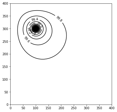
Plot a Map of Layer 1

hds = flopy.utils.binaryfile.HeadFile(headfile)
h = hds.get_data(kstpkper=(0, 0))
x = y = np.linspace(0, L, N)
y = y[::-1]
fig = plt.figure(figsize=(6, 6))
ax = fig.add_subplot(1, 1, 1, aspect="equal")
c = ax.contour(x, y, h[0], np.arange(90, 100.1, 0.2), colors="black")
plt.clabel(c, fmt="%2.1f")

<a list of 6 text.Text objects>

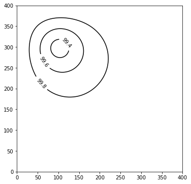
Plot a Map of Layer 10

x = y = np.linspace(0, L, N)
y = y[::-1]
fig = plt.figure(figsize=(6, 6))
ax = fig.add_subplot(1, 1, 1, aspect="equal")
c = ax.contour(x, y, h[-1], np.arange(90, 100.1, 0.2), colors="black")
plt.clabel(c, fmt="%1.1f")

<a list of 3 text.Text objects>

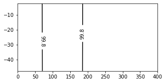
Plot a Cross-section along row 51

z = np.linspace(-H / Nlay / 2, -H + H / Nlay / 2, Nlay)
fig = plt.figure(figsize=(5, 2.5))
ax = fig.add_subplot(1, 1, 1, aspect="auto")
c = ax.contour(x, z, h[:, 50, :], np.arange(90, 100.1, 0.2), colors="black")
plt.clabel(c, fmt="%1.1f")

<a list of 2 text.Text objects>

We can also use the Flopy PlotMapView() capabilities for MODFLOW 6

Before we start we will create a MODFLOW-2005 ibound array to use to plot the locations of the constant heads.

ibd = np.ones((Nlay, N, N), dtype=np.int)
for k, i, j in ra["cellid"]:
    ibd[k, i, j] = -1

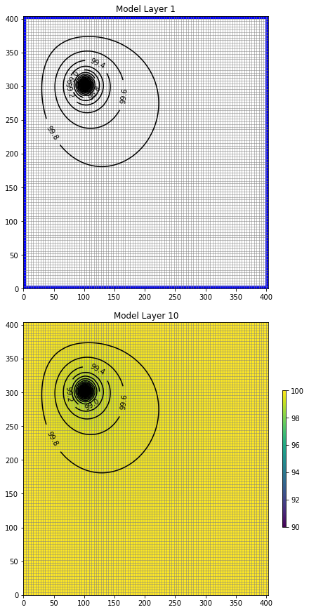
Plot a Map of Layers 1 and 10

fig, axes = plt.subplots(2, 1, figsize=(6, 12), constrained_layout=True)
# first subplot
ax = axes[0]
ax.set_title("Model Layer 1")
modelmap = flopy.plot.PlotMapView(model=gwf, ax=ax)
quadmesh = modelmap.plot_ibound(ibound=ibd)
linecollection = modelmap.plot_grid(lw=0.5, color="0.5")
contours = modelmap.contour_array(
    h[0], levels=np.arange(90, 100.1, 0.2), colors="black"
)
ax.clabel(contours, fmt="%2.1f")
# second subplot
ax = axes[1]
ax.set_title("Model Layer {}".format(Nlay))
modelmap = flopy.plot.PlotMapView(model=gwf, ax=ax, layer=Nlay - 1)
quadmesh = modelmap.plot_ibound(ibound=ibd)
linecollection = modelmap.plot_grid(lw=0.5, color="0.5")
pa = modelmap.plot_array(h[0])
contours = modelmap.contour_array(
    h[0], levels=np.arange(90, 100.1, 0.2), colors="black"
)
cb = plt.colorbar(pa, shrink=0.5, ax=ax)
ax.clabel(contours, fmt="%2.1f")

<a list of 5 text.Text objects>