MODFLOW Tutorial 2: Unconfined Transient Flow Model

In this example, we will convert the tutorial 1 model into an unconfined, transient flow model with time varying boundaries. Instead of using constant heads for the left and right boundaries (by setting ibound to -1), we will use general head boundaries. We will have the model consider the following conditions:

• Initial conditions – head is 10.0 everywhere
• Period 1 (1 day) – steady state with left and right GHB stage = 10.
• Period 2 (100 days) – left GHB with stage = 10., right GHB with stage set to 0.
• Period 3 (100 days) – pumping well at model center with rate = -500., left and right GHB = 10., and 0.

We will start with selected model commands from the previous tutorial.

Getting Started

As shown in the previous MODFLOW tutorial, import flopy.

import numpy as np
import flopy

Creating the MODFLOW Model

Define the Model Extent, Grid Resolution, and Characteristics

Assign the model information

Lx = 1000.0
Ly = 1000.0
ztop = 10.0
zbot = -50.0
nlay = 1
nrow = 10
ncol = 10
delr = Lx / ncol
delc = Ly / nrow
delv = (ztop - zbot) / nlay
botm = np.linspace(ztop, zbot, nlay + 1)
hk = 1.0
vka = 1.0
sy = 0.1
ss = 1.0e-4
laytyp = 1

Variables for the BAS package Note that changes from the MODFLOW tutorial 1

ibound = np.ones((nlay, nrow, ncol), dtype=np.int32)
strt = 10.0 * np.ones((nlay, nrow, ncol), dtype=np.float32)

Define the Stress Periods

To create a model with multiple stress periods, we need to define nper, perlen, nstp, and steady. This is done in the following block in a manner that allows us to pass these variable directly to the discretization object:

nper = 3
perlen = [1, 100, 100]
nstp = [1, 100, 100]
steady = [True, False, False]

Create Time-Invariant Flopy Objects

With this information, we can now create the static flopy objects that do not change with time:

modelname = "tutorial2_mf"
mf = flopy.modflow.Modflow(modelname, exe_name="mf2005")
dis = flopy.modflow.ModflowDis(
    mf,
    nlay,
    nrow,
    ncol,
    delr=delr,
    delc=delc,
    top=ztop,
    botm=botm[1:],
    nper=nper,
    perlen=perlen,
    nstp=nstp,
    steady=steady,
)
bas = flopy.modflow.ModflowBas(mf, ibound=ibound, strt=strt)
lpf = flopy.modflow.ModflowLpf(
    mf, hk=hk, vka=vka, sy=sy, ss=ss, laytyp=laytyp, ipakcb=53
)
pcg = flopy.modflow.ModflowPcg(mf)

Transient General-Head Boundary Package

At this point, our model is ready to add our transient boundary packages. First, we will create the GHB object, which is of the following type: flopy.modflow.ModflowGhb().

The key to creating Flopy transient boundary packages is recognizing that the boundary data is stored in a dictionary with key values equal to the zero-based stress period number and values equal to the boundary conditions for that stress period. For a GHB the values can be a two-dimensional nested list of [layer, row, column, stage, conductance].

stageleft = 10.0
stageright = 10.0
bound_sp1 = []
for il in range(nlay):
    condleft = hk * (stageleft - zbot) * delc
    condright = hk * (stageright - zbot) * delc
    for ir in range(nrow):
        bound_sp1.append([il, ir, 0, stageleft, condleft])
        bound_sp1.append([il, ir, ncol - 1, stageright, condright])
print("Adding ", len(bound_sp1), "GHBs for stress period 1.")

Adding  20 GHBs for stress period 1.

# Make list for stress period 2
stageleft = 10.0
stageright = 0.0
condleft = hk * (stageleft - zbot) * delc
condright = hk * (stageright - zbot) * delc
bound_sp2 = []
for il in range(nlay):
    for ir in range(nrow):
        bound_sp2.append([il, ir, 0, stageleft, condleft])
        bound_sp2.append([il, ir, ncol - 1, stageright, condright])
print("Adding ", len(bound_sp2), "GHBs for stress period 2.")

Adding  20 GHBs for stress period 2.

# We do not need to add a dictionary entry for stress period 3.
# Flopy will automatically take the list from stress period 2 and apply it
# to the end of the simulation
stress_period_data = {0: bound_sp1, 1: bound_sp2}

# Create the flopy ghb object
ghb = flopy.modflow.ModflowGhb(mf, stress_period_data=stress_period_data)

Transient Well Package

Now we can create the well package object, which is of the type, flopy.modflow.ModflowWel().

# Create the well package
# Remember to use zero-based layer, row, column indices!
pumping_rate = -500.0
wel_sp1 = [[0, nrow / 2 - 1, ncol / 2 - 1, 0.0]]
wel_sp2 = [[0, nrow / 2 - 1, ncol / 2 - 1, 0.0]]
wel_sp3 = [[0, nrow / 2 - 1, ncol / 2 - 1, pumping_rate]]
stress_period_data = {0: wel_sp1, 1: wel_sp2, 2: wel_sp3}
wel = flopy.modflow.ModflowWel(mf, stress_period_data=stress_period_data)

Output Control

Here we create the output control package object, which is of the type flopy.modflow.ModflowOc().

stress_period_data = {}
for kper in range(nper):
    for kstp in range(nstp[kper]):
        stress_period_data[(kper, kstp)] = [
            "save head",
            "save drawdown",
            "save budget",
            "print head",
            "print budget",
        ]
oc = flopy.modflow.ModflowOc(
    mf, stress_period_data=stress_period_data, compact=True
)

Running the Model

Run the model with the run_model method, which returns a success flag and the stream of output. With run_model, we have some finer control, that allows us to suppress the output.

# Write the model input files
mf.write_input()

# Run the model
success, mfoutput = mf.run_model(silent=True, pause=False)
if not success:
    raise Exception("MODFLOW did not terminate normally.")

Post-Processing the Results

Once again, we can read heads from the MODFLOW binary output file, using the flopy.utils.binaryfile() module. Included with the HeadFile object are several methods that we will use here:

• get_times() will return a list of times contained in the binary head file
• get_data() will return a three-dimensional head array for the specified time
• get_ts() will return a time series array [ntimes, headval] for the specified cell

Using these methods, we can create head plots and hydrographs from the model results.

# Imports
import matplotlib.pyplot as plt
import flopy.utils.binaryfile as bf

# Create the headfile and budget file objects
headobj = bf.HeadFile(modelname + ".hds")
times = headobj.get_times()
cbb = bf.CellBudgetFile(modelname + ".cbc")

# Setup contour parameters
levels = np.linspace(0, 10, 11)
extent = (delr / 2.0, Lx - delr / 2.0, delc / 2.0, Ly - delc / 2.0)
print("Levels: ", levels)
print("Extent: ", extent)

Levels:  [ 0.  1.  2.  3.  4.  5.  6.  7.  8.  9. 10.]
Extent:  (50.0, 950.0, 50.0, 950.0)

# Well point for plotting
wpt = (450.0, 550.0)

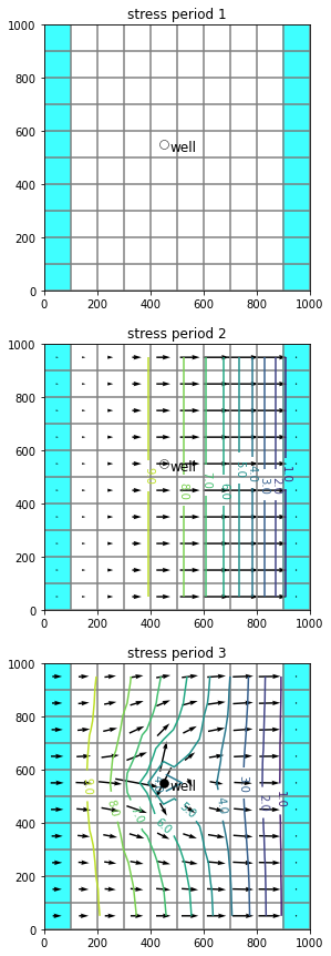
Create a figure with maps for three times

# Make the plots
fig = plt.figure(figsize=(5, 15))
mytimes = [1.0, 101.0, 201.0]
for iplot, time in enumerate(mytimes):
    print("*****Processing time: ", time)
    head = headobj.get_data(totim=time)
    # Print statistics
    print("Head statistics")
    print("  min: ", head.min())
    print("  max: ", head.max())
    print("  std: ", head.std())

    # Extract flow right face and flow front face
    frf = cbb.get_data(text="FLOW RIGHT FACE", totim=time)[0]
    fff = cbb.get_data(text="FLOW FRONT FACE", totim=time)[0]

    # Create a map for this time
    ax = fig.add_subplot(len(mytimes), 1, iplot + 1, aspect="equal")
    ax.set_title("stress period " + str(iplot + 1))

    pmv = flopy.plot.PlotMapView(model=mf, layer=0, ax=ax)
    qm = pmv.plot_ibound()
    lc = pmv.plot_grid()
    qm = pmv.plot_bc("GHB", alpha=0.5)
    if head.min() != head.max():
        cs = pmv.contour_array(head, levels=levels)
        plt.clabel(cs, inline=1, fontsize=10, fmt="%1.1f")
        quiver = pmv.plot_vector(frf, fff)

    mfc = "None"
    if (iplot + 1) == len(mytimes):
        mfc = "black"
    ax.plot(
        wpt[0],
        wpt[1],
        lw=0,
        marker="o",
        markersize=8,
        markeredgewidth=0.5,
        markeredgecolor="black",
        markerfacecolor=mfc,
        zorder=9,
    )
    ax.text(wpt[0] + 25, wpt[1] - 25, "well", size=12, zorder=12)

*****Processing time:  1.0
Head statistics
  min:  10.0
  max:  10.0
  std:  0.0
*****Processing time:  101.0
Head statistics
  min:  0.025931068
  max:  9.998436
  std:  3.2574987
*****Processing time:  201.0
Head statistics
  min:  0.016297927
  max:  9.994038
  std:  3.1544707

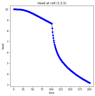
Create a hydrograph

# Plot the head versus time
idx = (0, int(nrow / 2) - 1, int(ncol / 2) - 1)
ts = headobj.get_ts(idx)
fig = plt.figure(figsize=(6, 6))
ax = fig.add_subplot(1, 1, 1)
ttl = "Head at cell ({0},{1},{2})".format(idx[0] + 1, idx[1] + 1, idx[2] + 1)
ax.set_title(ttl)
ax.set_xlabel("time")
ax.set_ylabel("head")
ax.plot(ts[:, 0], ts[:, 1], "bo-")

[<matplotlib.lines.Line2D at 0x7f0b119b0070>]