Note
a Jupyter notebook (.ipynb) or Python script (.py) or launch interactively with Binder MT3DMS Example Problems
The purpose of this notebook is to recreate the example problems that are described in the 1999 MT3DMS report.
There are 10 example problems: 1. One-Dimensional Transport in a Uniform Flow Field 2. One-Dimensional Transport with Nonlinear or Nonequilibrium Sorption 3. Two-Dimensional Transport in a Uniform Flow Field 4. Two-Dimensional Transport in a Diagonal Flow Field 5. Two-Dimensional Transport in a Radial Flow Field 6. Concentration at an Injection/Extraction Well 7. Three-Dimensional Transport in a Uniform Flow Field 8. Two-Dimensional, Vertical Transport in a Heterogeneous Aquifer 9. Two-Dimensional Application Example 10. Three-Dimensional Field Case Study
[1]:
import os
[2]:
import sys
from tempfile import TemporaryDirectory

import matplotlib as mpl
import matplotlib.pyplot as plt
import numpy as np

# run installed version of flopy or add local path
try:
    import flopy
except:
    fpth = os.path.abspath(os.path.join("..", ".."))
    sys.path.append(fpth)
    import flopy

from flopy.utils.util_array import read1d

mpl.rcParams["figure.figsize"] = (8, 8)

exe_name_mf = "mf2005"
exe_name_mt = "mt3dms"
datadir = os.path.join("..", "..", "examples", "data", "mt3d_test", "mt3dms")

# temporary directory
temp_dir = TemporaryDirectory()
workdir = temp_dir.name

print(sys.version)
print("numpy version: {}".format(np.__version__))
print("matplotlib version: {}".format(mpl.__version__))
print("flopy version: {}".format(flopy.__version__))
3.8.18 (default, Aug 28 2023, 08:27:22)
[GCC 11.4.0]
numpy version: 1.24.4
matplotlib version: 3.7.3
flopy version: 3.4.3
Example 1. One-Dimensional Transport in a Uniform Flow Field
This example has 4 cases: * Case 1a: Advection only * Case 1b: Advection and dispersion * Case 1c: Advection, dispersion, and sorption * Case 1d: Advection, dispersion, sorption, and decay
[3]:
def p01(dirname, al, retardation, lambda1, mixelm):
    model_ws = os.path.join(workdir, dirname)
    nlay = 1
    nrow = 1
    ncol = 101
    delr = 10
    delc = 1
    delv = 1
    Lx = (ncol - 1) * delr
    v = 0.24
    prsity = 0.25
    q = v * prsity

    perlen = 2000.0
    hk = 1.0
    laytyp = 0
    rhob = 0.25
    kd = (retardation - 1.0) * prsity / rhob

    modelname_mf = dirname + "_mf"
    mf = flopy.modflow.Modflow(
        modelname=modelname_mf, model_ws=model_ws, exe_name=exe_name_mf
    )
    dis = flopy.modflow.ModflowDis(
        mf,
        nlay=nlay,
        nrow=nrow,
        ncol=ncol,
        delr=delr,
        delc=delc,
        top=0.0,
        botm=[0 - delv],
        perlen=perlen,
    )
    ibound = np.ones((nlay, nrow, ncol), dtype=int)
    ibound[0, 0, 0] = -1
    ibound[0, 0, -1] = -1
    strt = np.zeros((nlay, nrow, ncol), dtype=float)
    h1 = q * Lx
    strt[0, 0, 0] = h1
    bas = flopy.modflow.ModflowBas(mf, ibound=ibound, strt=strt)
    lpf = flopy.modflow.ModflowLpf(mf, hk=hk, laytyp=laytyp)
    pcg = flopy.modflow.ModflowPcg(mf)
    lmt = flopy.modflow.ModflowLmt(mf)
    mf.write_input()
    success, buff = mf.run_model(silent=True, report=True)
    if success:
        for line in buff:
            print(line)
    else:
        raise ValueError("Failed to run.")

    modelname_mt = dirname + "_mt"
    mt = flopy.mt3d.Mt3dms(
        modelname=modelname_mt,
        model_ws=model_ws,
        exe_name=exe_name_mt,
        modflowmodel=mf,
    )
    c0 = 1.0
    icbund = np.ones((nlay, nrow, ncol), dtype=int)
    icbund[0, 0, 0] = -1
    sconc = np.zeros((nlay, nrow, ncol), dtype=float)
    sconc[0, 0, 0] = c0
    btn = flopy.mt3d.Mt3dBtn(mt, icbund=icbund, prsity=prsity, sconc=sconc)
    dceps = 1.0e-5
    nplane = 1
    npl = 0
    nph = 4
    npmin = 0
    npmax = 8
    nlsink = nplane
    npsink = nph
    adv = flopy.mt3d.Mt3dAdv(
        mt,
        mixelm=mixelm,
        dceps=dceps,
        nplane=nplane,
        npl=npl,
        nph=nph,
        npmin=npmin,
        npmax=npmax,
        nlsink=nlsink,
        npsink=npsink,
        percel=0.5,
    )
    dsp = flopy.mt3d.Mt3dDsp(mt, al=al)
    rct = flopy.mt3d.Mt3dRct(
        mt,
        isothm=1,
        ireact=1,
        igetsc=0,
        rhob=rhob,
        sp1=kd,
        rc1=lambda1,
        rc2=lambda1,
    )
    ssm = flopy.mt3d.Mt3dSsm(mt)
    gcg = flopy.mt3d.Mt3dGcg(mt)
    mt.write_input()
    fname = os.path.join(model_ws, "MT3D001.UCN")
    if os.path.isfile(fname):
        os.remove(fname)
    mt.run_model(silent=True)

    fname = os.path.join(model_ws, "MT3D001.UCN")
    ucnobj = flopy.utils.UcnFile(fname)
    times = ucnobj.get_times()
    conc = ucnobj.get_alldata()

    fname = os.path.join(model_ws, "MT3D001.OBS")
    if os.path.isfile(fname):
        cvt = mt.load_obs(fname)
    else:
        cvt = None

    fname = os.path.join(model_ws, "MT3D001.MAS")
    mvt = mt.load_mas(fname)

    return mf, mt, conc, cvt, mvt
[4]:
mf, mt, conc, cvt, mvt = p01("case1a", 0, 1, 0, 1)
x = mf.modelgrid.xcellcenters.ravel()
y = conc[0, 0, 0, :]
plt.plot(x, y, label="Case 1a")

mf, mt, conc, cvt, mvt = p01("case1b", 10, 1, 0, 1)
y = conc[0, 0, 0, :]
plt.plot(x, y, label="Case 1b")

mf, mt, conc, cvt, mvt = p01("case1c", 10, 5, 0, 2)
y = conc[0, 0, 0, :]
plt.plot(x, y, label="Case 1c")

mf, mt, conc, cvt, mvt = p01("case1d", 10, 5, 0.002, 2)
y = conc[0, 0, 0, :]
plt.plot(x, y, label="Case 1d")

plt.xlim(0, 1000)
plt.ylim(0, 1.2)
plt.xlabel("DISTANCE, IN METERS")
plt.ylabel("NORMALIZED CONCENTRATION, UNITLESS")
plt.legend()
                                  MODFLOW-2005
    U.S. GEOLOGICAL SURVEY MODULAR FINITE-DIFFERENCE GROUND-WATER FLOW MODEL
                             Version 1.12.00 2/3/2017

 Using NAME file: case1a_mf.nam
 Run start date and time (yyyy/mm/dd hh:mm:ss): 2023/09/30 20:45:58

 Solving:  Stress period:     1    Time step:     1    Ground-Water Flow Eqn.
 Run end date and time (yyyy/mm/dd hh:mm:ss): 2023/09/30 20:45:58
 Elapsed run time:  0.001 Seconds

  Normal termination of simulation

                                  MODFLOW-2005
    U.S. GEOLOGICAL SURVEY MODULAR FINITE-DIFFERENCE GROUND-WATER FLOW MODEL
                             Version 1.12.00 2/3/2017

 Using NAME file: case1b_mf.nam
 Run start date and time (yyyy/mm/dd hh:mm:ss): 2023/09/30 20:45:59

 Solving:  Stress period:     1    Time step:     1    Ground-Water Flow Eqn.
 Run end date and time (yyyy/mm/dd hh:mm:ss): 2023/09/30 20:45:59
 Elapsed run time:  0.001 Seconds

  Normal termination of simulation

                                  MODFLOW-2005
    U.S. GEOLOGICAL SURVEY MODULAR FINITE-DIFFERENCE GROUND-WATER FLOW MODEL
                             Version 1.12.00 2/3/2017

 Using NAME file: case1c_mf.nam
 Run start date and time (yyyy/mm/dd hh:mm:ss): 2023/09/30 20:45:59

 Solving:  Stress period:     1    Time step:     1    Ground-Water Flow Eqn.
 Run end date and time (yyyy/mm/dd hh:mm:ss): 2023/09/30 20:45:59
 Elapsed run time:  0.001 Seconds

  Normal termination of simulation

                                  MODFLOW-2005
    U.S. GEOLOGICAL SURVEY MODULAR FINITE-DIFFERENCE GROUND-WATER FLOW MODEL
                             Version 1.12.00 2/3/2017

 Using NAME file: case1d_mf.nam
 Run start date and time (yyyy/mm/dd hh:mm:ss): 2023/09/30 20:45:59

 Solving:  Stress period:     1    Time step:     1    Ground-Water Flow Eqn.
 Run end date and time (yyyy/mm/dd hh:mm:ss): 2023/09/30 20:45:59
 Elapsed run time:  0.001 Seconds

  Normal termination of simulation
[4]:
<matplotlib.legend.Legend at 0x7f05412db8b0>

[5]:
mf, mt, conc, cvt, mvt = p01("case1e", 0, 1, 0, 1)
y = conc[0, 0, 0, :]
plt.plot(x, y, label="MOC")

mf, mt, conc, cvt, mvt = p01("case1f", 0, 1, 0, -1)
y = conc[0, 0, 0, :]
plt.plot(x, y, label="ULTIMATE")

mf, mt, conc, cvt, mvt = p01("case1g", 0, 1, 0, 0)
y = conc[0, 0, 0, :]
plt.plot(x, y, label="Upstream FD")

plt.xlim(0, 1000)
plt.ylim(0, 1.2)
plt.xlabel("DISTANCE, IN METERS")
plt.ylabel("NORMALIZED CONCENTRATION, UNITLESS")
plt.legend()
                                  MODFLOW-2005
    U.S. GEOLOGICAL SURVEY MODULAR FINITE-DIFFERENCE GROUND-WATER FLOW MODEL
                             Version 1.12.00 2/3/2017

 Using NAME file: case1e_mf.nam
 Run start date and time (yyyy/mm/dd hh:mm:ss): 2023/09/30 20:45:59

 Solving:  Stress period:     1    Time step:     1    Ground-Water Flow Eqn.
 Run end date and time (yyyy/mm/dd hh:mm:ss): 2023/09/30 20:45:59
 Elapsed run time:  0.002 Seconds

  Normal termination of simulation

                                  MODFLOW-2005
    U.S. GEOLOGICAL SURVEY MODULAR FINITE-DIFFERENCE GROUND-WATER FLOW MODEL
                             Version 1.12.00 2/3/2017

 Using NAME file: case1f_mf.nam
 Run start date and time (yyyy/mm/dd hh:mm:ss): 2023/09/30 20:45:59

 Solving:  Stress period:     1    Time step:     1    Ground-Water Flow Eqn.
 Run end date and time (yyyy/mm/dd hh:mm:ss): 2023/09/30 20:45:59
 Elapsed run time:  0.002 Seconds

  Normal termination of simulation

                                  MODFLOW-2005
    U.S. GEOLOGICAL SURVEY MODULAR FINITE-DIFFERENCE GROUND-WATER FLOW MODEL
                             Version 1.12.00 2/3/2017

 Using NAME file: case1g_mf.nam
 Run start date and time (yyyy/mm/dd hh:mm:ss): 2023/09/30 20:45:59

 Solving:  Stress period:     1    Time step:     1    Ground-Water Flow Eqn.
 Run end date and time (yyyy/mm/dd hh:mm:ss): 2023/09/30 20:45:59
 Elapsed run time:  0.002 Seconds

  Normal termination of simulation
[5]:
<matplotlib.legend.Legend at 0x7f0541282c10>

[6]:
mf, mt, conc, cvt, mvt = p01("case1e", 10, 1, 0, 1)
y = conc[0, 0, 0, :]
plt.plot(x, y, label="MOC")

mf, mt, conc, cvt, mvt = p01("case1f", 10, 1, 0, -1)
y = conc[0, 0, 0, :]
plt.plot(x, y, label="ULTIMATE")

mf, mt, conc, cvt, mvt = p01("case1g", 10, 1, 0, 0)
y = conc[0, 0, 0, :]
plt.plot(x, y, label="Upstream FD")

plt.xlim(0, 1000)
plt.ylim(0, 1.2)
plt.xlabel("DISTANCE, IN METERS")
plt.ylabel("NORMALIZED CONCENTRATION, UNITLESS")
plt.legend()
                                  MODFLOW-2005
    U.S. GEOLOGICAL SURVEY MODULAR FINITE-DIFFERENCE GROUND-WATER FLOW MODEL
                             Version 1.12.00 2/3/2017

 Using NAME file: case1e_mf.nam
 Run start date and time (yyyy/mm/dd hh:mm:ss): 2023/09/30 20:45:59

 Solving:  Stress period:     1    Time step:     1    Ground-Water Flow Eqn.
 Run end date and time (yyyy/mm/dd hh:mm:ss): 2023/09/30 20:45:59
 Elapsed run time:  0.002 Seconds

  Normal termination of simulation

                                  MODFLOW-2005
    U.S. GEOLOGICAL SURVEY MODULAR FINITE-DIFFERENCE GROUND-WATER FLOW MODEL
                             Version 1.12.00 2/3/2017

 Using NAME file: case1f_mf.nam
 Run start date and time (yyyy/mm/dd hh:mm:ss): 2023/09/30 20:46:00

 Solving:  Stress period:     1    Time step:     1    Ground-Water Flow Eqn.
 Run end date and time (yyyy/mm/dd hh:mm:ss): 2023/09/30 20:46:00
 Elapsed run time:  0.002 Seconds

  Normal termination of simulation

                                  MODFLOW-2005
    U.S. GEOLOGICAL SURVEY MODULAR FINITE-DIFFERENCE GROUND-WATER FLOW MODEL
                             Version 1.12.00 2/3/2017

 Using NAME file: case1g_mf.nam
 Run start date and time (yyyy/mm/dd hh:mm:ss): 2023/09/30 20:46:00

 Solving:  Stress period:     1    Time step:     1    Ground-Water Flow Eqn.
 Run end date and time (yyyy/mm/dd hh:mm:ss): 2023/09/30 20:46:00
 Elapsed run time:  0.001 Seconds

  Normal termination of simulation
[6]:
<matplotlib.legend.Legend at 0x7f0540e04190>

Example 2. One-Dimensional Transport with Nonlinear or Nonequilibrium Sorption
[7]:
def p02(dirname, isothm, sp1, sp2, mixelm):
    model_ws = os.path.join(workdir, dirname)
    nlay = 1
    nrow = 1
    ncol = 101
    delr = 0.16
    delc = 1
    delv = 1
    Lx = (ncol - 1) * delr
    v = 0.1
    prsity = 0.37
    q = v * prsity

    perlen_mf = 1.0
    perlen_mt = [160, 1320]
    hk = 1.0
    laytyp = 0
    rhob = 1.587

    modelname_mf = dirname + "_mf"
    mf = flopy.modflow.Modflow(
        modelname=modelname_mf, model_ws=model_ws, exe_name=exe_name_mf
    )
    dis = flopy.modflow.ModflowDis(
        mf,
        nlay=nlay,
        nrow=nrow,
        ncol=ncol,
        delr=delr,
        delc=delc,
        top=0.0,
        botm=[0 - delv],
        perlen=perlen_mf,
    )
    ibound = np.ones((nlay, nrow, ncol), dtype=int)
    ibound[0, 0, 0] = -1
    ibound[0, 0, -1] = -1
    strt = np.zeros((nlay, nrow, ncol), dtype=float)
    h1 = q * Lx
    strt[0, 0, 0] = h1
    bas = flopy.modflow.ModflowBas(mf, ibound=ibound, strt=strt)
    lpf = flopy.modflow.ModflowLpf(mf, hk=hk, laytyp=laytyp)
    pcg = flopy.modflow.ModflowPcg(mf)
    lmt = flopy.modflow.ModflowLmt(mf)
    mf.write_input()
    mf.run_model(silent=True)

    modelname_mt = dirname + "_mt"
    mt = flopy.mt3d.Mt3dms(
        modelname=modelname_mt,
        model_ws=model_ws,
        exe_name=exe_name_mt,
        modflowmodel=mf,
    )
    btn = flopy.mt3d.Mt3dBtn(
        mt,
        icbund=1,
        prsity=prsity,
        sconc=0,
        nper=2,
        perlen=perlen_mt,
        obs=[(0, 0, 50)],
    )
    dceps = 1.0e-5
    nplane = 1
    npl = 0
    nph = 4
    npmin = 0
    npmax = 8
    nlsink = nplane
    npsink = nph
    adv = flopy.mt3d.Mt3dAdv(
        mt,
        mixelm=mixelm,
        dceps=dceps,
        nplane=nplane,
        npl=npl,
        nph=nph,
        npmin=npmin,
        npmax=npmax,
        nlsink=nlsink,
        npsink=npsink,
        percel=0.5,
    )
    al = 1.0
    dsp = flopy.mt3d.Mt3dDsp(mt, al=al)
    rct = flopy.mt3d.Mt3dRct(
        mt, isothm=isothm, ireact=0, igetsc=0, rhob=rhob, sp1=sp1, sp2=sp2
    )
    c0 = 0.05
    spd = {0: [0, 0, 0, c0, 1], 1: [0, 0, 0, 0.0, 1]}
    ssm = flopy.mt3d.Mt3dSsm(mt, stress_period_data=spd)
    gcg = flopy.mt3d.Mt3dGcg(mt)
    mt.write_input()
    fname = os.path.join(model_ws, "MT3D001.UCN")
    if os.path.isfile(fname):
        os.remove(fname)
    mt.run_model(silent=True)

    fname = os.path.join(model_ws, "MT3D001.UCN")
    ucnobj = flopy.utils.UcnFile(fname)
    times = ucnobj.get_times()
    conc = ucnobj.get_alldata()

    fname = os.path.join(model_ws, "MT3D001.OBS")
    if os.path.isfile(fname):
        cvt = mt.load_obs(fname)
    else:
        cvt = None

    fname = os.path.join(model_ws, "MT3D001.MAS")
    mvt = mt.load_mas(fname)

    return mf, mt, conc, cvt, mvt
[8]:
mf, mt, conc, cvt, mvt = p02("freundlich", 2, 0.3, 0.7, -1)
x = cvt["time"]
y = cvt["(1, 1, 51)"] / 0.05
plt.plot(x, y, label="Freundlich")
plt.xlim(0, 1500)
plt.ylim(0, 0.5)
plt.xlabel("TIME, IN SECONDS")
plt.ylabel("NORMALIZED CONCENTRATION, UNITLESS")
plt.legend()
[8]:
<matplotlib.legend.Legend at 0x7f0540de6a90>

[9]:
mf, mt, conc, cvt, mvt = p02("langmuir", 3, 100.0, 0.003, -1)
x = cvt["time"]
y = cvt["(1, 1, 51)"] / 0.05
plt.plot(x, y, label="Langmuir")
plt.xlim(0, 500)
plt.ylim(0, 1.0)
plt.xlabel("TIME, IN SECONDS")
plt.ylabel("NORMALIZED CONCENTRATION, UNITLESS")
plt.legend()
[9]:
<matplotlib.legend.Legend at 0x7f0540dc38b0>

[10]:
for beta in [0, 2.0e-3, 1.0e-2, 20.0]:
    lbl = "beta={}".format(beta)
    mf, mt, conc, cvt, mvt = p02("nonequilibrium", 4, 0.933, beta, -1)
    x = cvt["time"]
    y = cvt["(1, 1, 51)"] / 0.05
    plt.plot(x, y, label=lbl)
plt.xlim(0, 1500)
plt.ylim(0, 1.0)
plt.xlabel("TIME, IN SECONDS")
plt.ylabel("NORMALIZED CONCENTRATION, UNITLESS")
plt.legend()
[10]:
<matplotlib.legend.Legend at 0x7f0540db7e80>

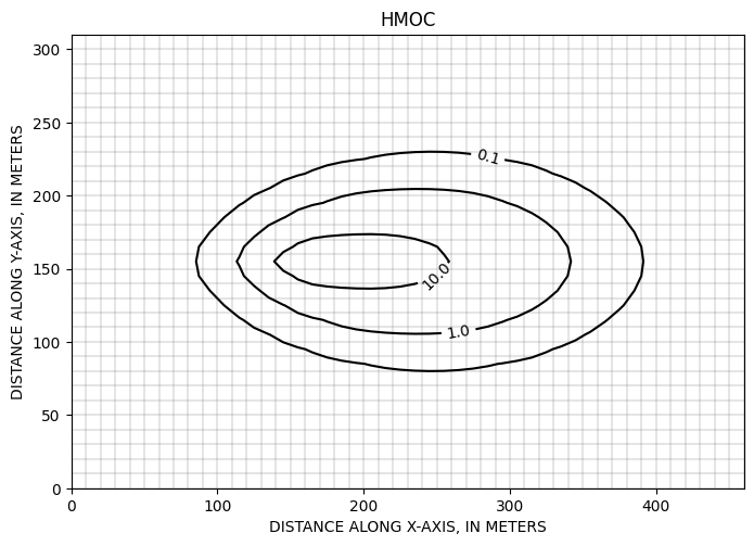
Example 3. Two-Dimensional Transport in a Uniform Flow Field
[11]:
def p03(dirname, mixelm):
    model_ws = os.path.join(workdir, dirname)
    nlay = 1
    nrow = 31
    ncol = 46
    delr = 10
    delc = 10
    delv = 10
    Lx = (ncol - 1) * delr
    v = 1.0 / 3.0
    prsity = 0.3
    q = v * prsity
    al = 10.0
    trpt = 0.3
    q0 = 1.0
    c0 = 1000.0

    perlen_mf = 365.0
    perlen_mt = 365.0
    hk = 1.0
    laytyp = 0

    modelname_mf = dirname + "_mf"
    mf = flopy.modflow.Modflow(
        modelname=modelname_mf, model_ws=model_ws, exe_name=exe_name_mf
    )
    dis = flopy.modflow.ModflowDis(
        mf,
        nlay=nlay,
        nrow=nrow,
        ncol=ncol,
        delr=delr,
        delc=delc,
        top=0.0,
        botm=[0 - delv],
        perlen=perlen_mf,
    )
    ibound = np.ones((nlay, nrow, ncol), dtype=int)
    ibound[0, :, 0] = -1
    ibound[0, :, -1] = -1
    strt = np.zeros((nlay, nrow, ncol), dtype=float)
    h1 = q * Lx
    strt[0, :, 0] = h1
    bas = flopy.modflow.ModflowBas(mf, ibound=ibound, strt=strt)
    lpf = flopy.modflow.ModflowLpf(mf, hk=hk, laytyp=laytyp)
    wel = flopy.modflow.ModflowWel(mf, stress_period_data=[[0, 15, 15, q0]])
    pcg = flopy.modflow.ModflowPcg(mf)
    lmt = flopy.modflow.ModflowLmt(mf)
    mf.write_input()
    mf.run_model(silent=True)

    modelname_mt = dirname + "_mt"
    mt = flopy.mt3d.Mt3dms(
        modelname=modelname_mt,
        model_ws=model_ws,
        exe_name=exe_name_mt,
        modflowmodel=mf,
    )
    btn = flopy.mt3d.Mt3dBtn(mt, icbund=1, prsity=prsity, sconc=0)
    dceps = 1.0e-5
    nplane = 1
    npl = 0
    nph = 16
    npmin = 2
    npmax = 32
    dchmoc = 1.0e-3
    nlsink = nplane
    npsink = nph
    adv = flopy.mt3d.Mt3dAdv(
        mt,
        mixelm=mixelm,
        dceps=dceps,
        nplane=nplane,
        npl=npl,
        nph=nph,
        npmin=npmin,
        npmax=npmax,
        nlsink=nlsink,
        npsink=npsink,
        percel=0.5,
    )
    dsp = flopy.mt3d.Mt3dDsp(mt, al=al, trpt=trpt)
    spd = {0: [0, 15, 15, c0, 2]}
    ssm = flopy.mt3d.Mt3dSsm(mt, stress_period_data=spd)
    gcg = flopy.mt3d.Mt3dGcg(mt)
    mt.write_input()
    fname = os.path.join(model_ws, "MT3D001.UCN")
    if os.path.isfile(fname):
        os.remove(fname)
    mt.run_model(silent=True)

    fname = os.path.join(model_ws, "MT3D001.UCN")
    ucnobj = flopy.utils.UcnFile(fname)
    times = ucnobj.get_times()
    conc = ucnobj.get_alldata()

    fname = os.path.join(model_ws, "MT3D001.OBS")
    if os.path.isfile(fname):
        cvt = mt.load_obs(fname)
    else:
        cvt = None

    fname = os.path.join(model_ws, "MT3D001.MAS")
    mvt = mt.load_mas(fname)

    return mf, mt, conc, cvt, mvt
[12]:
ax = plt.subplot(1, 1, 1, aspect="equal")
mf, mt, conc, cvt, mvt = p03("p03", 3)
conc = conc[0, :, :, :]
pmv = flopy.plot.PlotMapView(model=mf)
pmv.plot_grid(color=".5", alpha=0.2)
cs = pmv.contour_array(conc, levels=[0.1, 1.0, 10.0, 50.0], colors="k")
plt.clabel(cs)
plt.xlabel("DISTANCE ALONG X-AXIS, IN METERS")
plt.ylabel("DISTANCE ALONG Y-AXIS, IN METERS")
plt.title("HMOC")
[12]:
Text(0.5, 1.0, 'HMOC')
[13]:
ax = plt.subplot(1, 1, 1, aspect="equal")
mf, mt, conc, cvt, mvt = p03("p03", -1)
conc = conc[0, :, :, :]
pmv = flopy.plot.PlotMapView(model=mf)
pmv.plot_grid(color=".5", alpha=0.2)
cs = pmv.contour_array(conc, levels=[0.1, 1.0, 10.0, 50.0], colors="k")
plt.clabel(cs)
plt.xlabel("DISTANCE ALONG X-AXIS, IN METERS")
plt.ylabel("DISTANCE ALONG Y-AXIS, IN METERS")
plt.title("ULTIMATE")
[13]:
Text(0.5, 1.0, 'ULTIMATE')

Example 4. Two-Dimensional Transport in a Diagonal Flow Field
[14]:
def p04(dirname, mixelm):
    model_ws = os.path.join(workdir, dirname)
    nlay = 1
    nrow = 100
    ncol = 100
    delr = 10
    delc = 10
    delv = 1
    Lx = (ncol - 1) * delr
    Ly = (nrow - 1) * delc
    Ls = np.sqrt(Lx**2 + Ly**2)
    v = 1.0
    prsity = 0.14
    q = v * prsity
    al = 2.0
    trpt = 0.1
    q0 = 0.01
    c0 = 1000.0

    perlen_mf = 1000.0
    perlen_mt = 1000.0
    hk = 1.0
    laytyp = 0

    modelname_mf = dirname + "_mf"
    mf = flopy.modflow.Modflow(
        modelname=modelname_mf, model_ws=model_ws, exe_name=exe_name_mf
    )
    dis = flopy.modflow.ModflowDis(
        mf,
        nlay=nlay,
        nrow=nrow,
        ncol=ncol,
        delr=delr,
        delc=delc,
        top=0.0,
        botm=[0 - delv],
        perlen=perlen_mf,
    )
    ibound = np.ones((nlay, nrow, ncol), dtype=int) * -1
    ibound[:, 1 : nrow - 1, 1 : ncol - 1] = 1

    # set strt as a linear gradient at a 45 degree angle
    h1 = q * Ls
    x = mf.modelgrid.xcellcenters
    y = mf.modelgrid.ycellcenters
    a = -1
    b = -1
    c = 1
    d = abs(a * x + b * y + c) / np.sqrt(2)
    strt = h1 - d / Ls * h1

    bas = flopy.modflow.ModflowBas(mf, ibound=ibound, strt=strt)
    lpf = flopy.modflow.ModflowLpf(mf, hk=hk, laytyp=laytyp)
    wel = flopy.modflow.ModflowWel(mf, stress_period_data=[[0, 79, 20, q0]])
    pcg = flopy.modflow.ModflowPcg(mf)
    lmt = flopy.modflow.ModflowLmt(mf)
    mf.write_input()
    mf.run_model(silent=True)

    modelname_mt = dirname + "_mt"
    mt = flopy.mt3d.Mt3dms(
        modelname=modelname_mt,
        model_ws=model_ws,
        exe_name=exe_name_mt,
        modflowmodel=mf,
    )
    btn = flopy.mt3d.Mt3dBtn(mt, icbund=1, prsity=prsity, sconc=0)
    dceps = 1.0e-5
    nplane = 1
    npl = 0
    nph = 16
    npmin = 2
    npmax = 32
    dchmoc = 1.0e-3
    nlsink = nplane
    npsink = nph
    adv = flopy.mt3d.Mt3dAdv(
        mt,
        mixelm=mixelm,
        dceps=dceps,
        nplane=nplane,
        npl=npl,
        nph=nph,
        npmin=npmin,
        npmax=npmax,
        nlsink=nlsink,
        npsink=npsink,
        percel=0.5,
    )
    dsp = flopy.mt3d.Mt3dDsp(mt, al=al, trpt=trpt)
    spd = {0: [0, 79, 20, c0, 2]}
    ssm = flopy.mt3d.Mt3dSsm(mt, stress_period_data=spd)
    gcg = flopy.mt3d.Mt3dGcg(mt)
    mt.write_input()
    fname = os.path.join(model_ws, "MT3D001.UCN")
    if os.path.isfile(fname):
        os.remove(fname)
    mt.run_model(silent=True)

    fname = os.path.join(model_ws, "MT3D001.UCN")
    ucnobj = flopy.utils.UcnFile(fname)
    times = ucnobj.get_times()
    conc = ucnobj.get_alldata()

    fname = os.path.join(model_ws, "MT3D001.OBS")
    if os.path.isfile(fname):
        cvt = mt.load_obs(fname)
    else:
        cvt = None

    fname = os.path.join(model_ws, "MT3D001.MAS")
    mvt = mt.load_mas(fname)

    return mf, mt, conc, cvt, mvt
[15]:
ax = plt.subplot(1, 1, 1, aspect="equal")
mf, mt, conc, cvt, mvt = p04("p04", 1)
grid = mf.modelgrid
conc = conc[0, :, :, :]
levels = [0.1, 1.0, 1.5, 2.0, 5.0]
pmv = flopy.plot.PlotMapView(model=mf)
cf = plt.contourf(grid.xcellcenters, grid.ycellcenters, conc[0], levels=levels)
plt.colorbar(cf, shrink=0.5)
cs = pmv.contour_array(conc, levels=levels, colors="k")
plt.clabel(cs)
plt.xlabel("DISTANCE ALONG X-AXIS, IN METERS")
plt.ylabel("DISTANCE ALONG Y-AXIS, IN METERS")
plt.title("MOC")
[15]:
Text(0.5, 1.0, 'MOC')

[16]:
ax = plt.subplot(1, 1, 1, aspect="equal")
mf, mt, conc, cvt, mvt = p04("p04", 0)
grid = mf.modelgrid
conc = conc[0, :, :, :]
levels = [0.1, 1.0, 1.5, 2.0, 5.0]
pmv = flopy.plot.PlotMapView(model=mf)
cf = plt.contourf(grid.xcellcenters, grid.ycellcenters, conc[0], levels=levels)
plt.colorbar(cf, shrink=0.5)
cs = pmv.contour_array(conc, levels=levels, colors="k")
plt.clabel(cs)
plt.xlabel("DISTANCE ALONG X-AXIS, IN METERS")
plt.ylabel("DISTANCE ALONG Y-AXIS, IN METERS")
plt.title("Upstream FD")
[16]:
Text(0.5, 1.0, 'Upstream FD')

[17]:
ax = plt.subplot(1, 1, 1, aspect="equal")
mf, mt, conc, cvt, mvt = p04("p04", -1)
grid = mf.modelgrid
conc = conc[0, :, :, :]
levels = [0.1, 1.0, 1.5, 2.0, 5.0]
pmv = flopy.plot.PlotMapView(model=mf)
cf = plt.contourf(grid.xcellcenters, grid.ycellcenters, conc[0], levels=levels)
plt.colorbar(cf, shrink=0.5)
cs = pmv.contour_array(conc, levels=levels, colors="k")
plt.clabel(cs)
plt.xlabel("DISTANCE ALONG X-AXIS, IN METERS")
plt.ylabel("DISTANCE ALONG Y-AXIS, IN METERS")
plt.title("ULTIMATE")
[17]:
Text(0.5, 1.0, 'ULTIMATE')

Example 5. Two-Dimensional Transport in a Radial Flow Field
[18]:
def p05(dirname, mixelm, dt0, ttsmult):
    model_ws = os.path.join(workdir, dirname)
    nlay = 1
    nrow = 31
    ncol = 31
    delr = 10
    delc = 10
    delv = 1
    prsity = 0.30
    al = 10.0
    trpt = 1.0
    q0 = 100.0
    c0 = 1.0

    perlen_mf = 27.0
    perlen_mt = 27.0
    hk = 1.0
    laytyp = 0

    modelname_mf = dirname + "_mf"
    mf = flopy.modflow.Modflow(
        modelname=modelname_mf, model_ws=model_ws, exe_name=exe_name_mf
    )
    dis = flopy.modflow.ModflowDis(
        mf,
        nlay=nlay,
        nrow=nrow,
        ncol=ncol,
        delr=delr,
        delc=delc,
        top=0.0,
        botm=[0 - delv],
        perlen=perlen_mf,
    )
    ibound = np.ones((nlay, nrow, ncol), dtype=int) * -1
    ibound[:, 1 : nrow - 1, 1 : ncol - 1] = 1
    strt = 0.0

    bas = flopy.modflow.ModflowBas(mf, ibound=ibound, strt=strt)
    lpf = flopy.modflow.ModflowLpf(mf, hk=hk, laytyp=laytyp)
    wel = flopy.modflow.ModflowWel(mf, stress_period_data=[[0, 15, 15, q0]])
    sip = flopy.modflow.ModflowSip(mf)
    lmt = flopy.modflow.ModflowLmt(mf)
    mf.write_input()
    mf.run_model(silent=True)

    modelname_mt = dirname + "_mt"
    mt = flopy.mt3d.Mt3dms(
        modelname=modelname_mt,
        model_ws=model_ws,
        exe_name=exe_name_mt,
        modflowmodel=mf,
    )
    btn = flopy.mt3d.Mt3dBtn(
        mt, icbund=1, prsity=prsity, sconc=0, dt0=dt0, ttsmult=ttsmult
    )
    dceps = 1.0e-5
    nplane = 1
    npl = 0
    nph = 16
    npmin = 2
    npmax = 32
    dchmoc = 1.0e-3
    nlsink = nplane
    npsink = nph
    adv = flopy.mt3d.Mt3dAdv(
        mt,
        mixelm=mixelm,
        dceps=dceps,
        nplane=nplane,
        npl=npl,
        nph=nph,
        npmin=npmin,
        npmax=npmax,
        nlsink=nlsink,
        npsink=npsink,
        percel=0.5,
    )
    dsp = flopy.mt3d.Mt3dDsp(mt, al=al, trpt=trpt)
    spd = {0: [0, 15, 15, c0, -1]}
    ssm = flopy.mt3d.Mt3dSsm(mt, stress_period_data=spd)
    gcg = flopy.mt3d.Mt3dGcg(mt)
    mt.write_input()
    fname = os.path.join(model_ws, "MT3D001.UCN")
    if os.path.isfile(fname):
        os.remove(fname)
    mt.run_model(silent=True)

    fname = os.path.join(model_ws, "MT3D001.UCN")
    ucnobj = flopy.utils.UcnFile(fname)
    times = ucnobj.get_times()
    conc = ucnobj.get_alldata()

    fname = os.path.join(model_ws, "MT3D001.OBS")
    if os.path.isfile(fname):
        cvt = mt.load_obs(fname)
    else:
        cvt = None

    fname = os.path.join(model_ws, "MT3D001.MAS")
    mvt = mt.load_mas(fname)

    return mf, mt, conc, cvt, mvt
[19]:
mf, mt, conc, cvt, mvt = p05("p05", -1, 0.3, 1.0)
grid = mf.modelgrid
conc = conc[0, 0, :, :]
x = grid.xcellcenters[15, 15:] - grid.xcellcenters[15, 15]
y = conc[15, 15:]
plt.plot(x, y, label="ULTIMATE", marker="o")

mf, mt, conc, cvt, mvt = p05("p05", 0, 0.3, 1.0)
conc = conc[0, 0, :, :]
x = grid.xcellcenters[15, 15:] - grid.xcellcenters[15, 15]
y = conc[15, 15:]
plt.plot(x, y, label="Upstream FD (TTSMULT=1.0)", marker="^")

mf, mt, conc, cvt, mvt = p05("p05", 0, 0.3, 1.5)
conc = conc[0, 0, :, :]
x = grid.xcellcenters[15, 15:] - grid.xcellcenters[15, 15]
y = conc[15, 15:]
plt.plot(x, y, label="Upstream FD (TTSMULT=1.5)", marker="^")

plt.xlabel("RADIAL DISTANCE FROM THE SOURCE, IN METERS")
plt.ylabel("NORMALIZED CONCENTRATION, UNITLESS")
plt.legend()
[19]:
<matplotlib.legend.Legend at 0x7f053c4a9f40>

[20]:
ax = plt.subplot(1, 1, 1, aspect="equal")
mf, mt, conc, cvt, mvt = p05("p05", -1, 0.3, 1.0)
pmv = flopy.plot.PlotMapView(model=mf)
pmv.plot_grid(color=".5", alpha=0.2)
pmv.plot_ibound()
cs = pmv.contour_array(conc[0])
plt.clabel(cs)
plt.xlabel("DISTANCE ALONG X-AXIS, IN METERS")
plt.ylabel("DISTANCE ALONG Y-AXIS, IN METERS")
plt.title("ULTIMATE")
[20]:
Text(0.5, 1.0, 'ULTIMATE')

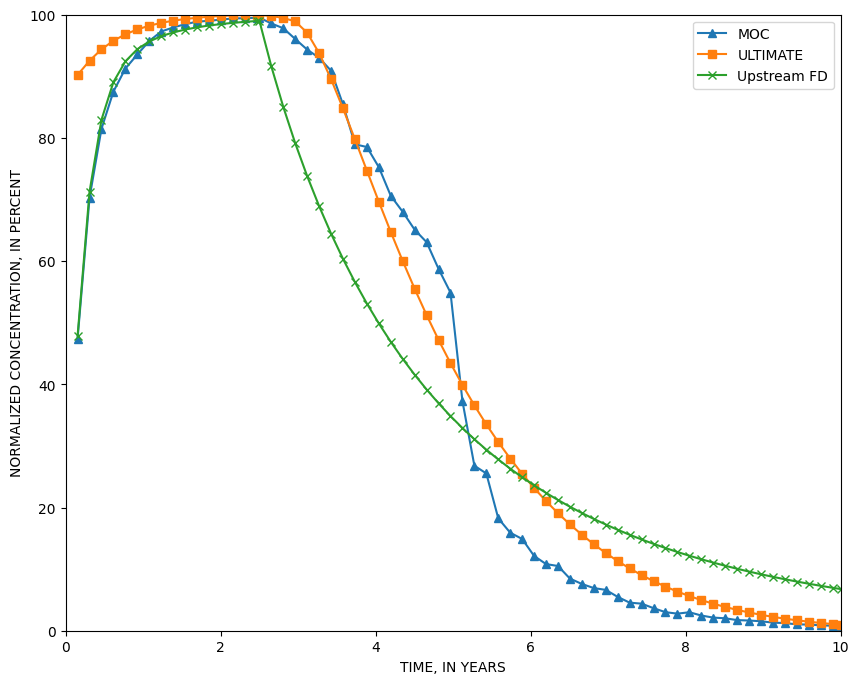
Example 6. Concentration at an Injection/Extraction Well
[21]:
def p06(dirname, mixelm, dt0):
    model_ws = os.path.join(workdir, dirname)
    nlay = 1
    nrow = 31
    ncol = 31
    delr = 900
    delc = 900
    delv = 20
    prsity = 0.30
    al = 100.0
    trpt = 1.0
    q0 = 86400.0
    c0 = 100.0

    perlen_mf = [912.5, 2737.5]
    perlen_mt = perlen_mf
    hk = 0.005 * 86400
    laytyp = 0

    modelname_mf = dirname + "_mf"
    mf = flopy.modflow.Modflow(
        modelname=modelname_mf, model_ws=model_ws, exe_name=exe_name_mf
    )
    dis = flopy.modflow.ModflowDis(
        mf,
        nlay=nlay,
        nrow=nrow,
        ncol=ncol,
        delr=delr,
        delc=delc,
        top=0.0,
        botm=[0 - delv],
        nper=2,
        perlen=perlen_mf,
    )
    ibound = np.ones((nlay, nrow, ncol), dtype=int) * -1
    ibound[:, 1 : nrow - 1, 1 : ncol - 1] = 1
    strt = 0.0

    bas = flopy.modflow.ModflowBas(mf, ibound=ibound, strt=strt)
    lpf = flopy.modflow.ModflowLpf(mf, hk=hk, laytyp=laytyp)
    welspd = {0: [[0, 15, 15, q0]], 1: [[0, 15, 15, -q0]]}
    wel = flopy.modflow.ModflowWel(mf, stress_period_data=welspd)
    sip = flopy.modflow.ModflowSip(mf)
    lmt = flopy.modflow.ModflowLmt(mf)
    mf.write_input()
    mf.run_model(silent=True)

    modelname_mt = dirname + "_mt"
    mt = flopy.mt3d.Mt3dms(
        modelname=modelname_mt,
        model_ws=model_ws,
        exe_name=exe_name_mt,
        modflowmodel=mf,
    )
    btn = flopy.mt3d.Mt3dBtn(
        mt,
        icbund=1,
        prsity=prsity,
        sconc=0,
        nper=2,
        perlen=perlen_mt,
        dt0=dt0,
        obs=[(0, 15, 15)],
    )
    dceps = 1.0e-5
    nplane = 1
    npl = 16
    nph = 16
    npmin = 4
    npmax = 32
    dchmoc = 1.0e-3
    nlsink = nplane
    npsink = nph
    adv = flopy.mt3d.Mt3dAdv(
        mt,
        mixelm=mixelm,
        dceps=dceps,
        nplane=nplane,
        npl=npl,
        nph=nph,
        npmin=npmin,
        npmax=npmax,
        nlsink=nlsink,
        npsink=npsink,
        percel=0.5,
    )
    dsp = flopy.mt3d.Mt3dDsp(mt, al=al, trpt=trpt)
    spd = {0: [0, 15, 15, c0, 2], 1: [0, 15, 15, 0.0, 2]}
    ssm = flopy.mt3d.Mt3dSsm(mt, stress_period_data=spd)
    gcg = flopy.mt3d.Mt3dGcg(mt)
    mt.write_input()
    fname = os.path.join(model_ws, "MT3D001.UCN")
    if os.path.isfile(fname):
        os.remove(fname)
    mt.run_model(silent=True)

    fname = os.path.join(model_ws, "MT3D001.UCN")
    ucnobj = flopy.utils.UcnFile(fname)
    times = ucnobj.get_times()
    conc = ucnobj.get_alldata()

    fname = os.path.join(model_ws, "MT3D001.OBS")
    if os.path.isfile(fname):
        cvt = mt.load_obs(fname)
    else:
        cvt = None

    fname = os.path.join(model_ws, "MT3D001.MAS")
    mvt = mt.load_mas(fname)

    return mf, mt, conc, cvt, mvt
[22]:
fig = plt.figure(figsize=(10, 8))
ax = fig.add_subplot(1, 1, 1)
mf, mt, conc, cvt, mvt = p06("p06", 1, 56.25)
x = cvt["time"] / 365.0
y = cvt["(1, 16, 16)"]
ax.plot(x, y, label="MOC", marker="^")

mf, mt, conc, cvt, mvt = p06("p06", -1, 56.25)
x = cvt["time"] / 365.0
y = cvt["(1, 16, 16)"]
ax.plot(x, y, label="ULTIMATE", marker="s")

mf, mt, conc, cvt, mvt = p06("p06", 0, 56.25)
x = cvt["time"] / 365.0
y = cvt["(1, 16, 16)"]
ax.plot(x, y, label="Upstream FD", marker="x")

plt.xlim(0, 10)
plt.ylim(0, 100.0)
plt.xlabel("TIME, IN YEARS")
plt.ylabel("NORMALIZED CONCENTRATION, IN PERCENT")
plt.legend()
[22]:
<matplotlib.legend.Legend at 0x7f053c314eb0>
Example 7. Three-Dimensional Transport in a Uniform Flow Field
[23]:
def p07(dirname, mixelm):
    model_ws = os.path.join(workdir, dirname)
    nlay = 8
    nrow = 15
    ncol = 21
    delr = 10
    delc = 10
    delv = 10
    Lx = (ncol - 1) * delr
    v = 1.0 / 3.0
    prsity = 0.2
    q = v * prsity
    al = 10.0
    trpt = 0.3
    trpv = 0.3
    q0 = 0.5
    c0 = 100.0

    perlen_mf = 100.0
    perlen_mt = 100.0
    hk = 0.5
    laytyp = 0

    modelname_mf = dirname + "_mf"
    mf = flopy.modflow.Modflow(
        modelname=modelname_mf, model_ws=model_ws, exe_name=exe_name_mf
    )
    dis = flopy.modflow.ModflowDis(
        mf,
        nlay=nlay,
        nrow=nrow,
        ncol=ncol,
        delr=delr,
        delc=delc,
        top=0.0,
        botm=[-delv * k for k in range(1, nlay + 1)],
        perlen=perlen_mf,
    )
    ibound = np.ones((nlay, nrow, ncol), dtype=int)
    ibound[:, :, 0] = -1
    ibound[:, :, -1] = -1
    strt = np.zeros((nlay, nrow, ncol), dtype=float)
    h1 = q * Lx
    strt[:, :, 0] = h1
    bas = flopy.modflow.ModflowBas(mf, ibound=ibound, strt=strt)
    lpf = flopy.modflow.ModflowLpf(mf, hk=hk, laytyp=laytyp)
    wel = flopy.modflow.ModflowWel(mf, stress_period_data=[[6, 7, 2, q0]])
    pcg = flopy.modflow.ModflowPcg(mf)
    lmt = flopy.modflow.ModflowLmt(mf)
    mf.write_input()
    mf.run_model(silent=True)

    modelname_mt = dirname + "_mt"
    mt = flopy.mt3d.Mt3dms(
        modelname=modelname_mt,
        model_ws=model_ws,
        exe_name=exe_name_mt,
        modflowmodel=mf,
    )
    btn = flopy.mt3d.Mt3dBtn(mt, icbund=1, prsity=prsity, sconc=0)
    dceps = 1.0e-5
    nplane = 1
    npl = 0
    nph = 16
    npmin = 2
    npmax = 32
    dchmoc = 1.0e-3
    nlsink = nplane
    npsink = nph
    adv = flopy.mt3d.Mt3dAdv(
        mt,
        mixelm=mixelm,
        dceps=dceps,
        nplane=nplane,
        npl=npl,
        nph=nph,
        npmin=npmin,
        npmax=npmax,
        nlsink=nlsink,
        npsink=npsink,
        percel=0.5,
    )
    dsp = flopy.mt3d.Mt3dDsp(mt, al=al, trpt=trpt, trpv=trpv)
    spd = {0: [6, 7, 2, c0, 2]}
    ssm = flopy.mt3d.Mt3dSsm(mt, stress_period_data=spd)
    gcg = flopy.mt3d.Mt3dGcg(mt)
    mt.write_input()
    fname = os.path.join(model_ws, "MT3D001.UCN")
    if os.path.isfile(fname):
        os.remove(fname)
    mt.run_model(silent=True)

    fname = os.path.join(model_ws, "MT3D001.UCN")
    ucnobj = flopy.utils.UcnFile(fname)
    times = ucnobj.get_times()
    conc = ucnobj.get_alldata()

    fname = os.path.join(model_ws, "MT3D001.OBS")
    if os.path.isfile(fname):
        cvt = mt.load_obs(fname)
    else:
        cvt = None

    fname = os.path.join(model_ws, "MT3D001.MAS")
    mvt = mt.load_mas(fname)

    return mf, mt, conc, cvt, mvt
[24]:
fig = plt.figure(figsize=(10, 20))
mf, mt, conc, cvt, mvt = p07("p07", -1)
conc = conc[0]

ax = fig.add_subplot(3, 1, 1, aspect="equal")
ilay = 4
pmv = flopy.plot.PlotMapView(ax=ax, model=mf, layer=ilay)
pmv.plot_grid(color=".5", alpha=0.2)
pmv.plot_ibound()
cs = pmv.contour_array(conc, levels=[0.01, 0.05, 0.15, 0.50], colors="k")
plt.clabel(cs)
plt.xlabel("DISTANCE ALONG X-AXIS, IN METERS")
plt.ylabel("DISTANCE ALONG Y-AXIS, IN METERS")
plt.title("LAYER {}".format(ilay + 1))

ax = fig.add_subplot(3, 1, 2, aspect="equal")
ilay = 5
pmv = flopy.plot.PlotMapView(ax=ax, model=mf, layer=ilay)
pmv.plot_grid(color=".5", alpha=0.2)
pmv.plot_ibound()
cs = pmv.contour_array(conc, levels=[0.01, 0.05, 0.15, 0.50], colors="k")
plt.clabel(cs)
plt.xlabel("DISTANCE ALONG X-AXIS, IN METERS")
plt.ylabel("DISTANCE ALONG Y-AXIS, IN METERS")
plt.title("LAYER {}".format(ilay + 1))

ax = fig.add_subplot(3, 1, 3, aspect="equal")
ilay = 6
pmv = flopy.plot.PlotMapView(ax=ax, model=mf, layer=ilay)
pmv.plot_grid(color=".5", alpha=0.2)
pmv.plot_ibound()
cs = pmv.contour_array(conc, levels=[0.01, 0.05, 0.15, 0.50], colors="k")
plt.clabel(cs)
plt.xlabel("DISTANCE ALONG X-AXIS, IN METERS")
plt.ylabel("DISTANCE ALONG Y-AXIS, IN METERS")
plt.title("LAYER {}".format(ilay + 1))
plt.plot(grid.xcellcenters[7, 2], grid.ycellcenters[7, 2], "ko")

plt.tight_layout()

Example 8. Two-Dimensional, Vertical Transport in a Heterogeneous Aquifer
[25]:
def p08(dirname, mixelm):
    model_ws = os.path.join(workdir, dirname)
    nlay = 27
    nrow = 1
    ncol = 50
    delr = 5
    delc = 1
    delv = 0.25
    prsity = 0.35
    al = 0.5
    trpt = 0.01
    trpv = 0.01
    dmcoef = 1.34e-5 / 100 / 100 * 86400
    rech = 0.1 / 365  # m/d

    perlen_mf = 1
    perlen_mt = [5 * 365, 15 * 365]

    k1 = 5e-4 / 100.0 * 86400  # m/d
    k2 = 1e-2 / 100.0 * 86400  # m/d
    hk = k1 * np.ones((nlay, nrow, ncol), dtype=float)
    hk[11:19, :, 0:24] = k2
    hk[11:19, :, 36:] = k2
    laytyp = 6 * [1] + 21 * [0]

    modelname_mf = dirname + "_mf"
    mf = flopy.modflow.Modflow(
        modelname=modelname_mf, model_ws=model_ws, exe_name=exe_name_mf
    )
    dis = flopy.modflow.ModflowDis(
        mf,
        nlay=nlay,
        nrow=nrow,
        ncol=ncol,
        delr=delr,
        delc=delc,
        top=6.75,
        botm=[6.75 - delv * k for k in range(1, nlay + 1)],
        perlen=perlen_mf,
    )
    f = open(os.path.join(datadir, "p08shead.dat"))
    strt = np.empty((nlay * ncol), dtype=float)
    strt = read1d(f, strt).reshape((nlay, nrow, ncol))
    f.close()
    ibound = np.ones((nlay, nrow, ncol), dtype=int)
    ibound[5:, :, -1] = -1
    ibound[strt < 0] = 0

    bas = flopy.modflow.ModflowBas(mf, ibound=ibound, strt=strt)
    lpf = flopy.modflow.ModflowLpf(mf, hk=hk, vka=hk, laytyp=laytyp)
    rch = flopy.modflow.ModflowRch(mf, rech=rech)
    pcg = flopy.modflow.ModflowPcg(mf)
    lmt = flopy.modflow.ModflowLmt(mf)
    mf.write_input()
    mf.run_model(silent=True)

    modelname_mt = dirname + "_mt"
    mt = flopy.mt3d.Mt3dms(
        modelname=modelname_mt,
        model_ws=model_ws,
        exe_name=exe_name_mt,
        modflowmodel=mf,
    )
    btn = flopy.mt3d.Mt3dBtn(
        mt,
        icbund=1,
        prsity=prsity,
        sconc=0,
        nper=2,
        perlen=perlen_mt,
        timprs=[8 * 365, 12 * 365, 20 * 365],
    )
    percel = 1.0
    itrack = 3
    wd = 0.5
    dceps = 1.0e-5
    nplane = 0
    npl = 0
    nph = 10
    npmin = 2
    npmax = 20
    dchmoc = 1.0e-3
    nlsink = nplane
    npsink = nph
    adv = flopy.mt3d.Mt3dAdv(
        mt,
        mixelm=mixelm,
        dceps=dceps,
        nplane=nplane,
        npl=npl,
        nph=nph,
        npmin=npmin,
        npmax=npmax,
        nlsink=nlsink,
        npsink=npsink,
        percel=percel,
        itrack=itrack,
        wd=wd,
    )
    dsp = flopy.mt3d.Mt3dDsp(mt, al=al, trpt=trpt, trpv=trpv, dmcoef=dmcoef)
    crch1 = np.zeros((nrow, ncol), dtype=float)
    crch1[0, 9:18] = 1.0
    cnc0 = [(0, 0, j, 1, -1) for j in range(8, 16)]
    cnc1 = [(0, 0, j, 0.0, -1) for j in range(8, 16)]
    ssmspd = {0: cnc0, 1: cnc1}
    ssm = flopy.mt3d.Mt3dSsm(mt, stress_period_data=ssmspd)
    gcg = flopy.mt3d.Mt3dGcg(mt)
    mt.write_input()
    fname = os.path.join(model_ws, "MT3D001.UCN")
    if os.path.isfile(fname):
        os.remove(fname)
    mt.run_model(silent=True)

    fname = os.path.join(model_ws, "MT3D001.UCN")
    ucnobj = flopy.utils.UcnFile(fname)
    times = ucnobj.get_times()
    conc = ucnobj.get_alldata()

    fname = os.path.join(model_ws, "MT3D001.OBS")
    if os.path.isfile(fname):
        cvt = mt.load_obs(fname)
    else:
        cvt = None

    fname = os.path.join(model_ws, "MT3D001.MAS")
    mvt = mt.load_mas(fname)

    return mf, mt, conc, cvt, mvt
[26]:
fig = plt.figure(figsize=(10, 15))
mf, mt, conc, cvt, mvt = p08("p08", 3)
hk = mf.lpf.hk.array

ax = fig.add_subplot(3, 1, 1)
mx = flopy.plot.PlotCrossSection(ax=ax, model=mf, line={"row": 0})
mx.plot_array(hk, masked_values=[hk[0, 0, 0]], alpha=0.2)
mx.plot_ibound()
mx.plot_grid(color="0.5", alpha=0.2)
cs = mx.contour_array(
    conc[1], levels=np.arange(0.05, 0.55, 0.05), masked_values=[1.0e30]
)
ax.set_title("TIME = 8 YEARS")

ax = fig.add_subplot(3, 1, 2)
mx = flopy.plot.PlotCrossSection(ax=ax, model=mf, line={"row": 0})
mx.plot_array(hk, masked_values=[hk[0, 0, 0]], alpha=0.2)
mx.plot_ibound()
mx.plot_grid(color="0.5", alpha=0.2)
cs = mx.contour_array(
    conc[2], levels=np.arange(0.05, 0.55, 0.05), masked_values=[1.0e30]
)
ax.set_title("TIME = 12 YEARS")

ax = fig.add_subplot(3, 1, 3)
mx = flopy.plot.PlotCrossSection(ax=ax, model=mf, line={"row": 0})
mx.plot_array(hk, masked_values=[hk[0, 0, 0]], alpha=0.2)
mx.plot_ibound()
mx.plot_grid(color="0.5", alpha=0.2)
cs = mx.contour_array(
    conc[3], levels=[0.05, 0.1, 0.15, 0.19], masked_values=[1.0e30]
)
ax.set_title("TIME = 20 YEARS")
found 'rch' in modflow model, resetting crch to 0.0
[26]:
Text(0.5, 1.0, 'TIME = 20 YEARS')

Example 9. Two-Dimensional Application Example
[27]:
def p09(dirname, mixelm, nadvfd):
    model_ws = os.path.join(workdir, dirname)
    nlay = 1
    nrow = 18
    ncol = 14
    delr = 100
    delc = 100
    delv = 10
    prsity = 0.3
    al = 20.0
    trpt = 0.2

    perlen_mf = 1.0
    perlen_mt = [365.0 * 86400, 365.0 * 86400]
    laytyp = 0
    k1 = 1.474e-4
    k2 = 1.474e-7
    hk = k1 * np.ones((nlay, nrow, ncol), dtype=float)
    hk[:, 5:8, 1:8] = k2

    modelname_mf = dirname + "_mf"
    mf = flopy.modflow.Modflow(
        modelname=modelname_mf, model_ws=model_ws, exe_name=exe_name_mf
    )
    dis = flopy.modflow.ModflowDis(
        mf,
        nlay=nlay,
        nrow=nrow,
        ncol=ncol,
        delr=delr,
        delc=delc,
        top=0.0,
        botm=[0 - delv],
        perlen=perlen_mf,
    )
    ibound = np.ones((nlay, nrow, ncol), dtype=int)
    ibound[0, 0, :] = -1
    ibound[0, -1, :] = -1
    strt = np.zeros((nlay, nrow, ncol), dtype=float)
    strt[0, 0, :] = 250.0
    xc = mf.modelgrid.xcellcenters
    for j in range(ncol):
        strt[0, -1, j] = 20.0 + (xc[0, j] - xc[0, 0]) * 2.5 / 100
    bas = flopy.modflow.ModflowBas(mf, ibound=ibound, strt=strt)
    lpf = flopy.modflow.ModflowLpf(mf, hk=hk, laytyp=laytyp)
    welspd = [[0, 3, 6, 0.001], [0, 10, 6, -0.0189]]
    wel = flopy.modflow.ModflowWel(mf, stress_period_data=welspd)
    pcg = flopy.modflow.ModflowPcg(mf)
    lmt = flopy.modflow.ModflowLmt(mf)
    mf.write_input()
    mf.run_model(silent=True)

    modelname_mt = dirname + "_mt"
    mt = flopy.mt3d.Mt3dms(
        modelname=modelname_mt,
        model_ws=model_ws,
        exe_name=exe_name_mt,
        modflowmodel=mf,
    )
    btn = flopy.mt3d.Mt3dBtn(
        mt,
        icbund=1,
        prsity=prsity,
        sconc=0,
        nper=2,
        perlen=perlen_mt,
        obs=[[0, 10, 6]],
    )
    percel = 1.0
    itrack = 2
    dceps = 1.0e-5
    nplane = 0
    npl = 0
    nph = 16
    npmin = 0
    npmax = 32
    dchmoc = 1.0e-3
    nlsink = nplane
    npsink = nph
    adv = flopy.mt3d.Mt3dAdv(
        mt,
        mixelm=mixelm,
        dceps=dceps,
        nplane=nplane,
        npl=npl,
        nph=nph,
        npmin=npmin,
        npmax=npmax,
        nlsink=nlsink,
        npsink=npsink,
        percel=percel,
        itrack=itrack,
        nadvfd=nadvfd,
    )
    dsp = flopy.mt3d.Mt3dDsp(mt, al=al, trpt=trpt)
    spd = {
        0: [[0, 3, 6, 57.87, 2], [0, 10, 6, 0.0, 2]],
        1: [[0, 3, 6, 0.0, 2], [0, 10, 6, 0.0, 2]],
    }
    ssm = flopy.mt3d.Mt3dSsm(mt, stress_period_data=spd)
    gcg = flopy.mt3d.Mt3dGcg(mt)
    mt.write_input()
    fname = os.path.join(model_ws, "MT3D001.UCN")
    if os.path.isfile(fname):
        os.remove(fname)
    mt.run_model(silent=True)

    fname = os.path.join(model_ws, "MT3D001.UCN")
    ucnobj = flopy.utils.UcnFile(fname)
    times = ucnobj.get_times()
    conc = ucnobj.get_alldata()

    fname = os.path.join(model_ws, "MT3D001.OBS")
    if os.path.isfile(fname):
        cvt = mt.load_obs(fname)
    else:
        cvt = None

    fname = os.path.join(model_ws, "MT3D001.MAS")
    mvt = mt.load_mas(fname)

    return mf, mt, conc, cvt, mvt
[28]:
fig = plt.figure(figsize=(15, 10))
levels = np.arange(0.2, 10, 0.2)

ax = fig.add_subplot(1, 2, 1, aspect="equal")
mf, mt, conc, cvt, mvt = p09("p09", 3, 1)
cvt["time"] / 365.0 / 86400.0
y = cvt["(1, 11, 7)"]
conc = conc[:, 0, :, :]
cflood = np.ma.masked_less_equal(conc, 0.2)
pmv = flopy.plot.PlotMapView(ax=ax, model=mf)
pmv.plot_grid(color=".5", alpha=0.2)
cs = pmv.plot_array(cflood[0], alpha=0.2, vmin=0, vmax=3)
cs = pmv.contour_array(conc[0], colors="k", levels=levels)
plt.clabel(cs)
plt.xlabel("DISTANCE ALONG X-AXIS, IN METERS")
plt.ylabel("DISTANCE ALONG Y-AXIS, IN METERS")
plt.title("HMOC")

ax = fig.add_subplot(1, 2, 2, aspect="equal")
mf, mt, conc, cvt, mvt = p09("p09", -1, 1)
cvt["time"] / 365.0 / 86400.0
y = cvt["(1, 11, 7)"]
conc = conc[:, 0, :, :]
cflood = np.ma.masked_less_equal(conc, 0.2)
pmv = flopy.plot.PlotMapView(ax=ax, model=mf)
pmv.plot_grid(color=".5", alpha=0.2)
cs = pmv.plot_array(cflood[0], alpha=0.2, vmin=0, vmax=3)
cs = pmv.contour_array(conc[0], colors="k", levels=levels)
plt.clabel(cs)
plt.xlabel("DISTANCE ALONG X-AXIS, IN METERS")
plt.ylabel("DISTANCE ALONG Y-AXIS, IN METERS")
plt.title("ULTIMATE")
[28]:
Text(0.5, 1.0, 'ULTIMATE')

[29]:
fig = plt.figure(figsize=(10, 8))
ax = fig.add_subplot(1, 1, 1)

mf, mt, conc, cvt, mvt = p09("p09", 3, 1)
x = cvt["time"] / 365.0 / 86400.0
y = cvt["(1, 11, 7)"]
plt.plot(x, y, label="HMOC", marker="d")

mf, mt, conc, cvt, mvt = p09("p09", -1, 1)
x = cvt["time"] / 365.0 / 86400.0
y = cvt["(1, 11, 7)"]
plt.plot(x, y, label="ULTIMATE", marker="^")

mf, mt, conc, cvt, mvt = p09("p09", 0, 1)
x = cvt["time"] / 365.0 / 86400.0
y = cvt["(1, 11, 7)"]
plt.plot(x, y, label="Upstream FD", marker="^")

mf, mt, conc, cvt, mvt = p09("p09", 0, 2)
x = cvt["time"] / 365.0 / 86400.0
y = cvt["(1, 11, 7)"]
plt.plot(x, y, label="Central FD", marker="^")

plt.xlim(0, 2)
plt.ylim(-0.2, 1.4)
plt.xlabel("TIME, IN YEARS")
plt.ylabel("CONCENTRATION, IN PPM")
plt.legend()
[29]:
<matplotlib.legend.Legend at 0x7f0535add790>

Example 10. Three-Dimensional Field Case Study
[30]:
def p10(dirname, mixelm, perlen=1000, isothm=1, sp2=0.0, ttsmult=1.2):
    model_ws = os.path.join(workdir, dirname)
    nlay = 4
    nrow = 61
    ncol = 40
    delr = (
        [2000, 1600, 800, 400, 200, 100]
        + 28 * [50]
        + [100, 200, 400, 800, 1600, 2000]
    )
    delc = (
        [2000, 2000, 2000, 1600, 800, 400, 200, 100]
        + 45 * [50]
        + [100, 200, 400, 800, 1600, 2000, 2000, 2000]
    )
    delv = 25.0
    top = 780.0
    botm = [top - delv * k for k in range(1, nlay + 1)]
    prsity = 0.3
    al = 10.0
    trpt = 0.2
    trpv = 0.2

    perlen_mf = perlen
    perlen_mt = perlen
    hk = [60.0, 60.0, 520.0, 520.0]
    vka = 0.1
    laytyp = 0

    modelname_mf = dirname + "_mf"
    mf = flopy.modflow.Modflow(
        modelname=modelname_mf, model_ws=model_ws, exe_name=exe_name_mf
    )
    dis = flopy.modflow.ModflowDis(
        mf,
        nlay=nlay,
        nrow=nrow,
        ncol=ncol,
        delr=delr,
        delc=delc,
        top=top,
        botm=botm,
        perlen=perlen_mf,
    )
    ibound = np.ones((nlay, nrow, ncol), dtype=int)

    # left side
    ibound[:, :, 0] = -1
    # right side
    ibound[:, :, -1] = -1
    # top
    ibound[:, 0, :] = -1
    # bottom
    ibound[:, -1, :] = -1

    f = open(os.path.join(datadir, "p10shead.dat"))
    s0 = np.empty((nrow * ncol), dtype=float)
    s0 = read1d(f, s0).reshape((nrow, ncol))
    f.close()
    strt = np.zeros((nlay, nrow, ncol), dtype=float)
    for k in range(nlay):
        strt[k] = s0
    bas = flopy.modflow.ModflowBas(mf, ibound=ibound, strt=strt)
    lpf = flopy.modflow.ModflowLpf(mf, hk=hk, layvka=1, vka=vka, laytyp=laytyp)
    welspd = [
        [3 - 1, 11 - 1, 29 - 1, -19230.00],
        [3 - 1, 19 - 1, 26 - 1, -19230.00],
        [3 - 1, 26 - 1, 23 - 1, -19230.00],
        [3 - 1, 33 - 1, 20 - 1, -19230.00],
        [3 - 1, 40 - 1, 17 - 1, -19230.00],
        [3 - 1, 48 - 1, 14 - 1, -19230.00],
        [3 - 1, 48 - 1, 9 - 1, -15384.00],
        [3 - 1, 52 - 1, 17 - 1, -17307.00],
    ]
    wel = flopy.modflow.ModflowWel(mf, stress_period_data=welspd)
    rch = flopy.modflow.ModflowRch(mf, rech=1.14e-3)
    pcg = flopy.modflow.ModflowPcg(mf)
    lmt = flopy.modflow.ModflowLmt(mf)
    mf.write_input()
    fname = os.path.join(model_ws, "MT3D001.UCN")
    if os.path.isfile(fname):
        os.remove(fname)
    mf.run_model(silent=True)

    modelname_mt = dirname + "_mt"
    mt = flopy.mt3d.Mt3dms(
        modelname=modelname_mt,
        model_ws=model_ws,
        exe_name=exe_name_mt,
        modflowmodel=mf,
    )
    f = open(os.path.join(datadir, "p10cinit.dat"))
    c0 = np.empty((nrow * ncol), dtype=float)
    c0 = read1d(f, c0).reshape((nrow, ncol))
    f.close()
    sconc = np.zeros((nlay, nrow, ncol), dtype=float)
    sconc[1] = 0.2 * c0
    sconc[2] = c0
    obs = [
        [3 - 1, 11 - 1, 29 - 1],
        [3 - 1, 19 - 1, 26 - 1],
        [3 - 1, 26 - 1, 23 - 1],
        [3 - 1, 33 - 1, 20 - 1],
        [3 - 1, 40 - 1, 17 - 1],
        [3 - 1, 48 - 1, 14 - 1],
        [3 - 1, 48 - 1, 9 - 1],
        [3 - 1, 52 - 1, 17 - 1],
    ]
    btn = flopy.mt3d.Mt3dBtn(
        mt,
        icbund=1,
        prsity=prsity,
        sconc=sconc,
        timprs=[500, 750, 1000],
        dt0=2.25,
        ttsmult=ttsmult,
        obs=obs,
    )
    dceps = 1.0e-5
    nplane = 0
    npl = 0
    nph = 16
    npmin = 2
    npmax = 32
    dchmoc = 0.01
    nlsink = nplane
    npsink = nph
    adv = flopy.mt3d.Mt3dAdv(
        mt,
        mixelm=mixelm,
        dceps=dceps,
        nplane=nplane,
        npl=npl,
        nph=nph,
        npmin=npmin,
        npmax=npmax,
        nlsink=nlsink,
        npsink=npsink,
        percel=1.0,
    )
    dsp = flopy.mt3d.Mt3dDsp(mt, al=al, trpt=trpt, trpv=trpv)
    ssm = flopy.mt3d.Mt3dSsm(mt, crch=0.0)
    rct = flopy.mt3d.Mt3dRct(
        mt, isothm=isothm, igetsc=0, rhob=1.7, sp1=0.176, sp2=sp2
    )
    mxiter = 1
    if isothm == 4:
        mxiter = 50
    gcg = flopy.mt3d.Mt3dGcg(mt, mxiter=mxiter, iter1=500)
    mt.write_input()
    fname = os.path.join(model_ws, "MT3D001.UCN")
    if os.path.isfile(fname):
        os.remove(fname)
    mt.run_model(silent=True)

    fname = os.path.join(model_ws, "MT3D001.UCN")
    ucnobj = flopy.utils.UcnFile(fname)
    times = ucnobj.get_times()
    conc = ucnobj.get_alldata()

    fname = os.path.join(model_ws, "MT3D001.OBS")
    if os.path.isfile(fname):
        cvt = mt.load_obs(fname)
    else:
        cvt = None

    fname = os.path.join(model_ws, "MT3D001.MAS")
    mvt = mt.load_mas(fname)

    return mf, mt, conc, cvt, mvt
[31]:
mf, mt, conctvd, cvttvd, mvttvd = p10("p10", -1)
mf, mt, conchmoc, cvthmoc, mvthmoc = p10("p10", 3)
mf, mt, concupfd, cvtupfd, mvtupfd = p10("p10", 0, ttsmult=1.0)
grid = mf.modelgrid
[32]:
fig = plt.figure(figsize=(10, 15))
ax = fig.add_subplot(2, 2, 1, aspect="equal")
cinit = mt.btn.sconc[0].array[2]
pmv = flopy.plot.PlotMapView(model=mf)
pmv.plot_grid(color=".5", alpha=0.2)
cs = pmv.contour_array(cinit, levels=np.arange(20, 200, 20))
plt.xlim(5100, 5100 + 28 * 50)
plt.ylim(9100, 9100 + 45 * 50)
plt.xlabel("DISTANCE ALONG X-AXIS, IN METERS")
plt.ylabel("DISTANCE ALONG Y-AXIS, IN METERS")
plt.title("LAYER {} INITIAL CONCENTRATION".format(3))
for k, i, j, q in mf.wel.stress_period_data[0]:
    plt.plot(grid.xcellcenters[i, j], grid.ycellcenters[i, j], "ks")

ax = fig.add_subplot(2, 2, 2, aspect="equal")
c = conctvd[0, 2]
chmoc = conchmoc[0, 2]
pmv = flopy.plot.PlotMapView(model=mf)
pmv.plot_grid(color=".5", alpha=0.2)
cs = pmv.contour_array(c, levels=np.arange(20, 200, 20))
cs = pmv.contour_array(chmoc, linestyles=":", levels=np.arange(20, 200, 20))
plt.xlim(5100, 5100 + 28 * 50)
plt.ylim(9100, 9100 + 45 * 50)
plt.xlabel("DISTANCE ALONG X-AXIS, IN METERS")
plt.ylabel("DISTANCE ALONG Y-AXIS, IN METERS")
plt.title("LAYER {} TIME = 500 DAYS".format(3))
for k, i, j, q in mf.wel.stress_period_data[0]:
    plt.plot(grid.xcellcenters[i, j], grid.ycellcenters[i, j], "ks")

ax = fig.add_subplot(2, 2, 3, aspect="equal")
c = conctvd[1, 2]
chmoc = conchmoc[1, 2]
pmv = flopy.plot.PlotMapView(model=mf)
pmv.plot_grid(color=".5", alpha=0.2)
cs = pmv.contour_array(c, levels=np.arange(20, 200, 20))
cs = pmv.contour_array(chmoc, linestyles=":", levels=np.arange(20, 200, 20))
plt.xlim(5100, 5100 + 28 * 50)
plt.ylim(9100, 9100 + 45 * 50)
plt.xlabel("DISTANCE ALONG X-AXIS, IN METERS")
plt.ylabel("DISTANCE ALONG Y-AXIS, IN METERS")
plt.title("LAYER {} TIME = 750 DAYS".format(3))
for k, i, j, q in mf.wel.stress_period_data[0]:
    plt.plot(grid.xcellcenters[i, j], grid.ycellcenters[i, j], "ks")

ax = fig.add_subplot(2, 2, 4, aspect="equal")
c = conctvd[2, 2]
chmoc = conchmoc[2, 2]
pmv = flopy.plot.PlotMapView(model=mf)
pmv.plot_grid(color=".5", alpha=0.2)
cs = pmv.contour_array(c, levels=np.arange(20, 200, 20))
cs = pmv.contour_array(chmoc, linestyles=":", levels=np.arange(20, 200, 20))
plt.xlim(5100, 5100 + 28 * 50)
plt.ylim(9100, 9100 + 45 * 50)
plt.xlabel("DISTANCE ALONG X-AXIS, IN METERS")
plt.ylabel("DISTANCE ALONG Y-AXIS, IN METERS")
plt.title("LAYER {} TIME = 1000 DAYS".format(3))
for k, i, j, q in mf.wel.stress_period_data[0]:
    plt.plot(grid.xcellcenters[i, j], grid.ycellcenters[i, j], "ks")

# plt.tight_layout()

[33]:
fig = plt.figure(figsize=(10, 8))
ax = fig.add_subplot(1, 1, 1)
w4 = "(3, 33, 20)"
ax.plot(cvthmoc["time"], cvthmoc[w4], "bd", label="HMOC")
ax.plot(cvtupfd["time"], cvtupfd[w4], "r+", label="Upstream FD")
ax.plot(cvttvd["time"], cvttvd[w4], "gx", label="ULTIMATE")
plt.xlim(0, 1000)
plt.ylim(0, 120)
plt.legend()
plt.xlabel("TIME, IN DAYS")
plt.ylabel("CONCENTRATION, IN PPB")
[33]:
Text(0, 0.5, 'CONCENTRATION, IN PPB')

[34]:
mf, mt, conctvd, cvttvd, mvt0 = p10("p10", 0, perlen=2000, isothm=0)
mf, mt, conctvd, cvttvd, mvt1 = p10("p10", 0, perlen=2000, isothm=1)
mf, mt, conctvd, cvttvd, mvt2 = p10("p10", 0, perlen=2000, isothm=4, sp2=0.1)
mf, mt, conctvd, cvttvd, mvt3 = p10(
    "p10", 0, perlen=2000, isothm=4, sp2=1.5e-4
)
mf, mt, conctvd, cvttvd, mvt4 = p10(
    "p10", 0, perlen=2000, isothm=4, sp2=1.0e-6
)
[35]:
fig = plt.figure(figsize=(10, 8))
ax = fig.add_subplot(1, 1, 1)
ax.plot(mvt0["time"], -mvt0["sinks"], "k--", label="No Sorption")
ax.plot(mvt1["time"], -mvt1["sinks"], "k-", label="Equilibrium Sorption")
ax.plot(
    mvt2["time"],
    -mvt2["sinks"],
    "k^",
    fillstyle="none",
    label="Nonequilibrium (rate=0.1 /day)",
)
ax.plot(
    mvt3["time"],
    -mvt3["sinks"],
    "ks",
    fillstyle="none",
    label="Nonequilibrium (rate=1.5e-4 /day)",
)
ax.plot(
    mvt4["time"],
    -mvt4["sinks"],
    "ko",
    fillstyle="none",
    label="Nonequilibrium (rate=1e-6 /day)",
)
plt.xlim(0, 2000)
plt.ylim(0, 5e9)
plt.legend(loc=2)
plt.xlabel("TIME, IN DAYS")
plt.ylabel("TOTAL MASS REMOVED")
[35]:
Text(0, 0.5, 'TOTAL MASS REMOVED')

[36]:
try:
    # ignore PermissionError on Windows
    temp_dir.cleanup()
except:
    pass