FloPy VTK/PyVista particle tracking pathline visualization demo
This notebook arranges and runs a steady state MODFLOW 6 groundwater flow model, then a MODPATH 7 particle tracking model, using the Freyberg grid. Particle tracks are exported to VTK files, then loaded and visualized with PyVista, first in a static plot and then an animated GIF.
First, import FloPy and show the version.
[1]:
import sys

import flopy

print(sys.version)
print(f"flopy version: {flopy.__version__}")
3.12.4 | packaged by conda-forge | (main, Jun 17 2024, 10:23:07) [GCC 12.3.0]
flopy version: 3.8.0
Load the Freyberg MF6 groundwater flow model.
[2]:
from pathlib import Path

from flopy.mf6 import MFSimulation

mdl_name = "freyberg"
sim_name = f"mf6-{mdl_name}-vtk-pathlines"
sim_path = Path.cwd().parent / "../examples/data" / f"mf6-{mdl_name}"

sim = MFSimulation.load(sim_name=sim_name, sim_ws=sim_path)
loading simulation...
  loading simulation name file...
  loading tdis package...
  loading model gwf6...
    loading package dis...
    loading package ic...
    loading package oc...
    loading package npf...
    loading package sto...
    loading package chd...
    loading package riv...
    loading package wel...
    loading package rch...
  loading solution package freyberg...
Create a temporary directory and change the simulation’s workspace.
[3]:
from tempfile import TemporaryDirectory

temp_path = TemporaryDirectory()
workspace = Path(temp_path.name)
sim.set_sim_path(workspace)
Write the input files to the temporary workspace.
[4]:
sim.write_simulation()
writing simulation...
  writing simulation name file...
  writing simulation tdis package...
  writing solution package freyberg...
  writing model freyberg...
    writing model name file...
    writing package dis...
    writing package ic...
    writing package oc...
    writing package npf...
    writing package sto...
    writing package chd-1...
    writing package riv-1...
    writing package wel-1...
    writing package rch-1...
Run the groundwater flow simulation.
[5]:
success, buff = sim.run_simulation(silent=True, report=True)
assert success, "MODFLOW 6 simulation failed"
for line in buff:
    print(line)
                                   MODFLOW 6
                U.S. GEOLOGICAL SURVEY MODULAR HYDROLOGIC MODEL
                  VERSION 6.6.0.dev0 (preliminary) 08/08/2024
                               ***DEVELOP MODE***

   MODFLOW 6 compiled Aug 08 2024 02:43:51 with Intel(R) Fortran Intel(R) 64
   Compiler Classic for applications running on Intel(R) 64, Version 2021.7.0
                             Build 20220726_000000

This software is preliminary or provisional and is subject to
revision. It is being provided to meet the need for timely best
science. The software has not received final approval by the U.S.
Geological Survey (USGS). No warranty, expressed or implied, is made
by the USGS or the U.S. Government as to the functionality of the
software and related material nor shall the fact of release
constitute any such warranty. The software is provided on the
condition that neither the USGS nor the U.S. Government shall be held
liable for any damages resulting from the authorized or unauthorized
use of the software.


 MODFLOW runs in SEQUENTIAL mode

 Run start date and time (yyyy/mm/dd hh:mm:ss): 2024/08/08 17:15:28

 Writing simulation list file: mfsim.lst
 Using Simulation name file: mfsim.nam

    Solving:  Stress period:     1    Time step:     1

 Run end date and time (yyyy/mm/dd hh:mm:ss): 2024/08/08 17:15:28
 Elapsed run time:  0.136 Seconds

 Normal termination of simulation.
Define particle release locations. In this example we will release 16 particles, with each particle released at the center of a unique grid cell. Cells containing particle release points are clustered into four 2x2 square regions.
[6]:
pgs = []
gwf = sim.get_model(mdl_name)

for i in range(1, 5):
    nrow = gwf.modelgrid.nrow
    ncol = gwf.modelgrid.ncol
    m = i * 2 if i < 3 else (nrow - i * 4)
    n = i * 2 if i < 3 else (ncol - i * 4)
    celldata = flopy.modpath.CellDataType(
        drape=0,
        columncelldivisions=1,
        rowcelldivisions=1,
        layercelldivisions=1,
    )
    lrcpd = flopy.modpath.LRCParticleData(
        subdivisiondata=[celldata],
        lrcregions=[[[0, m, n, 0, m + 1, n + 1]]],
    )
    pg = flopy.modpath.ParticleGroupLRCTemplate(
        particlegroupname=f"PG{i}",
        particledata=lrcpd,
        filename=f"{sim_name}.pg{i}.sloc",
    )
    pgs.append(pg)
Retrieve well locations (to define termination zones).
[7]:
import numpy as np

wel_locs = [
    (rec[0][1], rec[0][2]) for rec in (gwf.wel.stress_period_data.data[0])
]
print(wel_locs)
[(8, 15), (10, 12), (19, 13), (25, 9), (28, 5), (33, 11)]
Define particle termination zones.
[8]:
zone_maps = []


# zone 1 is the default (non-terminating regions)
def fill_zone_1():
    return np.ones((nrow, ncol), dtype=np.int32)


za = fill_zone_1()
for wl in wel_locs:
    za[wl] = 2  # wells
za[:, 14] = 3  # river is in column 14
zone_maps.append(za)
Create a MODPATH 7 simulation forward tracking model in combined (pathline & timeseries) mode.
[9]:
mp = flopy.modpath.Modpath7(
    modelname=f"{sim_name}_mp",
    flowmodel=gwf,
    exe_name="mp7",
    model_ws=workspace,
)
mpbas = flopy.modpath.Modpath7Bas(mp, porosity=0.1)
mpsim = flopy.modpath.Modpath7Sim(
    mp,
    simulationtype="combined",
    trackingdirection="forward",
    budgetoutputoption="summary",
    referencetime=[0, 0, 0.0],
    timepointdata=[1, [0]],
    zonedataoption="on",
    zones=zone_maps,
    particlegroups=pgs,
)
Write and run the particle tracking model.
[10]:
mp.write_input()
success, buff = mp.run_model(silent=True, report=True)
assert success, "MODPATH 7 simulation failed"
for line in buff:
    print(line)
MODPATH Version 7.2.001
Program compiled Jun 21 2024 03:00:39 with IFORT compiler (ver. 20.21.7)


Run particle tracking simulation ...
Processing Time Step     1 Period     1.  Time =  1.00000E+01  Steady-state flow

Particle Summary:
         0 particles are pending release.
         0 particles remain active.
         0 particles terminated at boundary faces.
        16 particles terminated at weak sink cells.
         0 particles terminated at weak source cells.
         0 particles terminated at strong source/sink cells.
         0 particles terminated in cells with a specified zone number.
         0 particles were stranded in inactive or dry cells.
         0 particles were unreleased.
         0 particles have an unknown status.

Normal termination.
Open the pathline output file and read pathline data.
[11]:
from flopy.utils import PathlineFile

pf = PathlineFile(workspace / mpsim.pathlinefilename)
pl = pf.get_alldata()
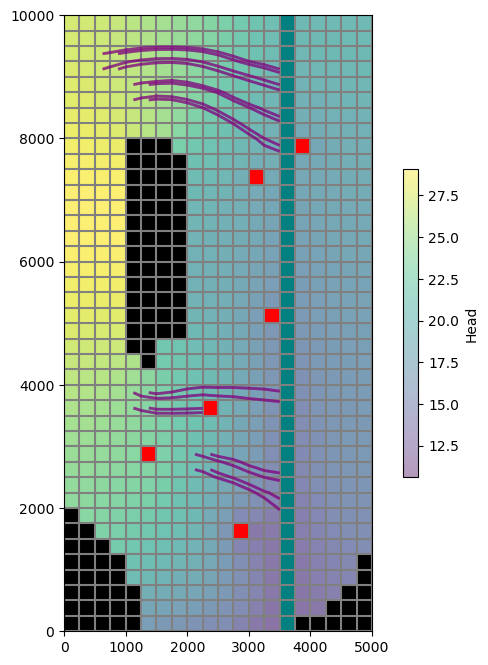
Plot the grid, heads, boundary conditions, and pathlines.
[12]:
import matplotlib.pyplot as plt

hf = flopy.utils.HeadFile(workspace / f"{mdl_name}.hds")
hds = hf.get_data()

fig = plt.figure(figsize=(8, 8))
ax = fig.add_subplot(1, 1, 1, aspect="equal")
mv = flopy.plot.PlotMapView(model=gwf)
mv.plot_grid()
mv.plot_ibound()
hd = mv.plot_array(hds, alpha=0.4)
cb = plt.colorbar(hd, shrink=0.5)
cb.set_label("Head")
mv.plot_bc("RIV")
mv.plot_bc("WEL", plotAll=True)
mv.plot_pathline(pl, layer="all", alpha=0.5, colors=["purple"], lw=2)
plt.show()
Create a Vtk object and add the flow model outputs and pathlines.
[13]:
from flopy.export.vtk import Vtk

vtk = Vtk(model=gwf, binary=False, vertical_exageration=50, smooth=False)
vtk.add_model(gwf)
vtk.add_pathline_points(pl)
Convert the VTK object to PyVista meshes.
[14]:
grid, pathlines = vtk.to_pyvista()
Rotate the meshes to match the orientation of the map view plot above.
[15]:
import pyvista as pv

axes = pv.Axes(show_actor=True, actor_scale=2.0, line_width=5)

grid.rotate_z(160, point=axes.origin, inplace=True)
pathlines.rotate_z(160, point=axes.origin, inplace=True)
[15]:
| Header | Data Arrays | ||||||||||||||||||||||||||||||||||||||||||||||||||||||||||||||||||||||||||||||||||||||||||||||||||||||||||||||
|---|---|---|---|---|---|---|---|---|---|---|---|---|---|---|---|---|---|---|---|---|---|---|---|---|---|---|---|---|---|---|---|---|---|---|---|---|---|---|---|---|---|---|---|---|---|---|---|---|---|---|---|---|---|---|---|---|---|---|---|---|---|---|---|---|---|---|---|---|---|---|---|---|---|---|---|---|---|---|---|---|---|---|---|---|---|---|---|---|---|---|---|---|---|---|---|---|---|---|---|---|---|---|---|---|---|---|---|---|---|---|---|
|
|
Check some grid properties to make sure the export succeeded.
[16]:
assert grid.n_cells == gwf.modelgrid.nnodes
print("Model grid has", grid.n_cells, "cells")
print("Model grid has", grid.n_arrays, "arrays")
Model grid has 800 cells
Model grid has 9 arrays
Select particle release locations and build a dictionary of particle tracks (pathlines). This will be used below for particle labelling, as well as for animation.
Note: while below we construct pathlines manually from data read from the exported VTK files, pathlines may also be read directly from the MODPATH 7 pathline output file (provided the simulation was run in pathline or combined mode, as this one was).
[17]:
tracks = {}
particle_ids = set()
release_locs = list()

for i, t in enumerate(pathlines["time"]):
    pid = str(round(float(pathlines["particleid"][i])))
    loc = pathlines.points[i]

    if pid not in tracks:
        tracks[pid] = []
        particle_ids.add(pid)
        release_locs.append(loc)

    # store the particle location in the corresponding track
    tracks[pid].append((loc, t))

release_locs = np.array(release_locs)
tracks = {k: np.array(v, dtype=object) for k, v in tracks.items()}
max_track_len = max([len(v) for v in tracks.values()])
print("The maximum number of locations per particle track is", max_track_len)
The maximum number of locations per particle track is 18
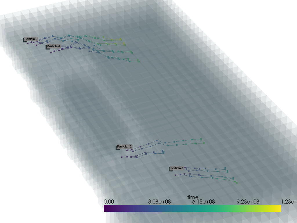
View the grid and pathlines with PyVista, with particle tracks/locations colored by time. Also add particle ID labels to a few particles’ release locations.
[18]:
pv.set_plot_theme("document")
pv.set_jupyter_backend("static")

# create the plot and add the grid and pathline meshes
p = pv.Plotter()
p.add_mesh(grid, opacity=0.05)
p.add_mesh(pathlines, scalars="time")

# add a particle ID label to each 4th particle's starting point
label_coords = []
start_labels = []
for pid, track in tracks.items():
    if int(pid) % 4 == 0:
        label_coords.append(track[0][0])
        start_labels.append(f"Particle {pid}")

p.add_point_labels(
    label_coords,
    start_labels,
    font_size=10,
    point_size=15,
    point_color="black",
)

# zoom in and show the plot
p.camera.zoom(2.4)
p.show()
Create an animated GIF of the particles traveling along their pathlines, with particles colored by time.
[19]:
# create plotter
p = pv.Plotter(notebook=False, off_screen=True)

# open GIF file
gif_path = workspace / f"{sim_name}_tracks.gif"
p.open_gif(str(gif_path))

# create mesh from release locations
spls = pv.PolyData(release_locs)
spls.point_data["time"] = np.zeros(len(spls.points))

# add the underlying grid mesh and particle data, then zoom in
p.add_mesh(grid, opacity=0.05)
p.add_mesh(spls, clim=[0, 1.23e09])
p.camera.zoom(2.4)

# cycle through time steps and update particle location
for i in range(1, max_track_len):
    pts = []
    times = []
    segments = []

    for pid in particle_ids:
        track = tracks[pid]
        npts = len(track)
        # use last locn if particle has already terminated
        loc, t = track[i] if i < npts else track[npts - 1]
        pts.append(loc)
        times.append(t)
        if i < npts:
            segments.append(track[i - 1][0])
            segments.append(loc)

    p.update_coordinates(np.vstack(pts), render=False)
    p.update_scalars(np.array(times), mesh=spls, render=False)
    p.add_lines(np.array(segments), width=1, color="black")
    p.write_frame()  # write frame to file

# close the plotter and the GIF file
p.close()
/home/runner/micromamba/envs/flopy/lib/python3.12/site-packages/pyvista/plotting/plotter.py:4872: PyVistaDeprecationWarning: This method is deprecated and will be removed in a future version of PyVista. Directly modify the points of a mesh in-place instead.
  warnings.warn(
/home/runner/micromamba/envs/flopy/lib/python3.12/site-packages/pyvista/plotting/plotter.py:4796: PyVistaDeprecationWarning: This method is deprecated and will be removed in a future version of PyVista. Directly modify the scalars of a mesh in-place instead.
  warnings.warn(
Show the GIF.
[20]:
from IPython.core.display import Image

display(Image(data=open(gif_path, "rb").read(), format="gif"))
<IPython.core.display.Image object>
Clean up the temporary workspace.
[21]:
try:
    # ignore PermissionError on Windows
    temp_path.cleanup()
except:
    pass