Intersecting rasters with modelgrids using FloPy’s Raster class
A Raster class was developed as a wrapper that leverages RasterIO, RasterStats, and SciPy built in methods for easy raster intersections and cropping.
This notebook will show some of the basic functionality of the Raster class with structured and unstructured model grid examples.
The Raster class accepts Tiff and GeoTiff, ASCII Grid (ESRI ASCII), and Erdas Imagine .img files.
Ideally this can be used to easily snap DEM rasters, PET, PPT, recharge and other rasters to a modflow grid for further processing and/or to apply as fluxes and boundary conditions to a MODFLOW model
[1]:
import os
import sys
import time
from tempfile import TemporaryDirectory

import matplotlib as mpl
import matplotlib.pyplot as plt
import numpy as np
import pandas as pd
import shapefile
import shapely

import flopy
from flopy.utils import Raster

print(sys.version)
print(f"numpy version: {np.__version__}")
print(f"matplotlib version: {mpl.__version__}")
print(f"pandas version: {pd.__version__}")
print(f"shapely version: {shapely.__version__}")
print(f"flopy version: {flopy.__version__}")
3.12.6 | packaged by conda-forge | (main, Sep 30 2024, 18:08:52) [GCC 13.3.0]
numpy version: 2.1.1
matplotlib version: 3.9.2
pandas version: 2.2.3
shapely version: 2.0.6
flopy version: 3.8.2
[2]:
# temporary directory
temp_dir = TemporaryDirectory()
workspace = temp_dir.name
Raster files can be loaded using the Raster.load method
[3]:
raster_ws = os.path.join("..", "..", "examples", "data", "options", "dem")
raster_name = "dem.img"

rio = Raster.load(os.path.join(raster_ws, raster_name))
The bands within the raster can be viewed by calling the parameter bands; there is only one band in this raster
[4]:
rio.bands
[4]:
(1,)
[5]:
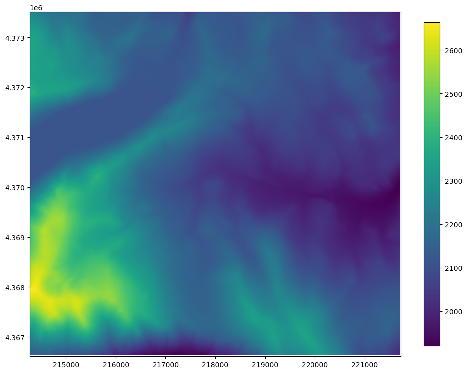
arr = rio.get_array(1)
idx = np.isfinite(arr)

vmin, vmax = arr[idx].min(), arr[idx].max()
vmin, vmax
[5]:
(np.float64(1920.5467529296875), np.float64(2663.162109375))
Using the built in .plot method, we can take a look at the DEM raster data before we start manipulating it
[6]:
fig = plt.figure(figsize=(12, 12))
ax = fig.add_subplot(1, 1, 1, aspect="equal")

ax = rio.plot(ax=ax, vmin=vmin, vmax=vmax)
plt.colorbar(ax.images[0], shrink=0.7)
[6]:
<matplotlib.colorbar.Colorbar at 0x7f99b2dc24e0>
Intersecting and resampling a data using the FloPy ModelGrid
Structured Grid Example
The structured grid example uses the DIS file from the GSFLOW Sagehen example problem to create a modelgrid
[7]:
model_ws = os.path.join("..", "..", "examples", "data", "options", "sagehen")
ml = flopy.modflow.Modflow.load(
    "sagehen.nam", version="mfnwt", model_ws=model_ws
)

xoff = 214110
yoff = 4366620
ml.modelgrid.set_coord_info(xoff=xoff, yoff=yoff)
   loading iuzfbnd array...
   loading vks array...
   loading eps array...
   loading thts array...
stress period 1:
   loading finf array...
stress period 2:
[8]:
fig = plt.figure(figsize=(12, 12))
ax = fig.add_subplot(1, 1, 1, aspect="equal")

ax = rio.plot(ax=ax, vmin=vmin, vmax=vmax)
plt.colorbar(ax.images[0], shrink=0.7)
pmv = flopy.plot.PlotMapView(modelgrid=ml.modelgrid)
pmv.plot_grid(ax=ax, lw=0.5, color="black")
[8]:
<matplotlib.collections.LineCollection at 0x7f99b2aa3d10>
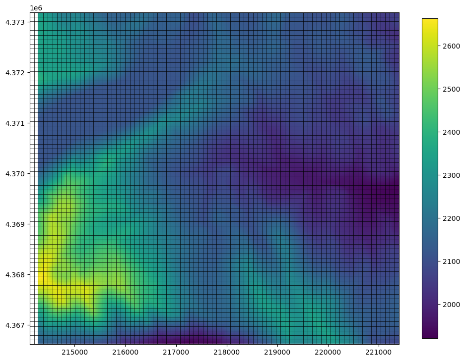
Once a modelgrid has been loaded, the resample_to_grid() method can be used to re-sample the data to an array consistent with the model grid.
Inputs to resample_to_grid() include:
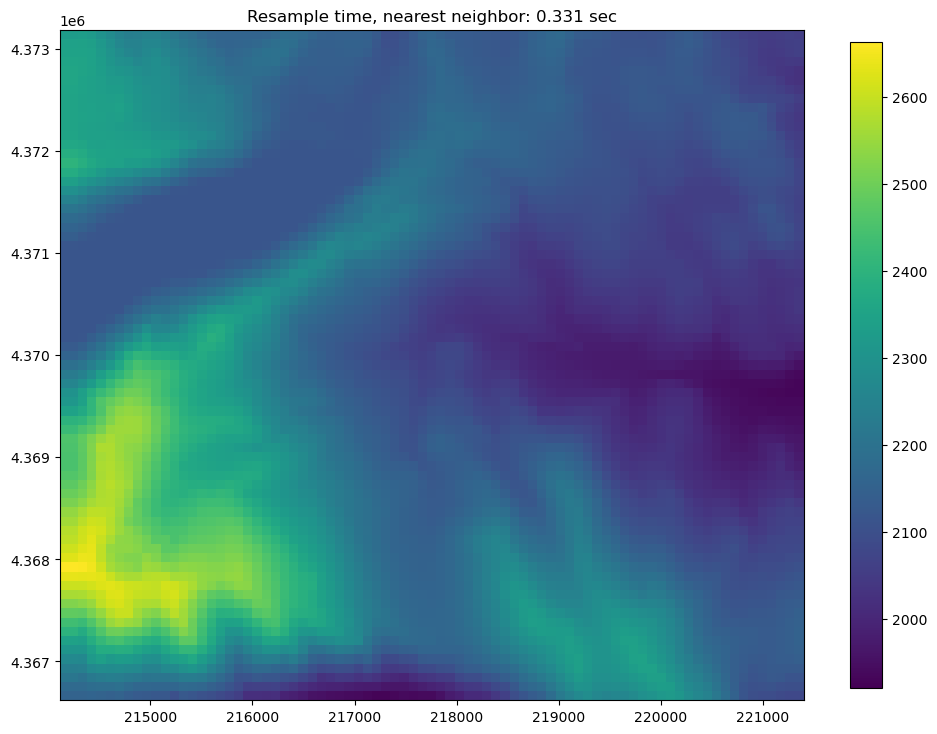
modelgrid: flopyGridobjectband: raster band to resamplemethod: resampling method, options include:"nearest"for nearest neighbor"linear"for bilinear sampling"cubic"for bicubic sampling"mean"for mean value sampling"median"for median value sampling"min"for minimum value sampling"max"for maximum value sampling"mode"for most often (dominant) sampling
extrapolate_edges: boolean flag to extrapolate edges using the"nearest"resampling method. For all of the sampling methods except"nearest", interpolation is only performed in areas bounded by data; nodata values are returned in areas without data. This option has no effect when the"nearest"interpolation method is used.
Note: Bottlenecks in sampling time depend on the resampling method used: + "nearest", "linear", and "cubic" bottlenecks are due to raster resolution. + "mean", "median", "min", "max", and "mode" are a function of the number of grid cells.
[9]:
t0 = time.time()
dem_data = rio.resample_to_grid(
    ml.modelgrid, band=rio.bands[0], method="nearest"
)
resample_time = time.time() - t0
[10]:
# now to visualize using flopy and matplotlib
fig = plt.figure(figsize=(12, 12))
ax = fig.add_subplot(1, 1, 1, aspect="equal")

pmv = flopy.plot.PlotMapView(modelgrid=ml.modelgrid, ax=ax)
ax = pmv.plot_array(
    dem_data, masked_values=rio.nodatavals, vmin=vmin, vmax=vmax
)
plt.title(f"Resample time, nearest neighbor: {resample_time:.3f} sec")
plt.colorbar(ax, shrink=0.7)
[10]:
<matplotlib.colorbar.Colorbar at 0x7f99a122ee70>
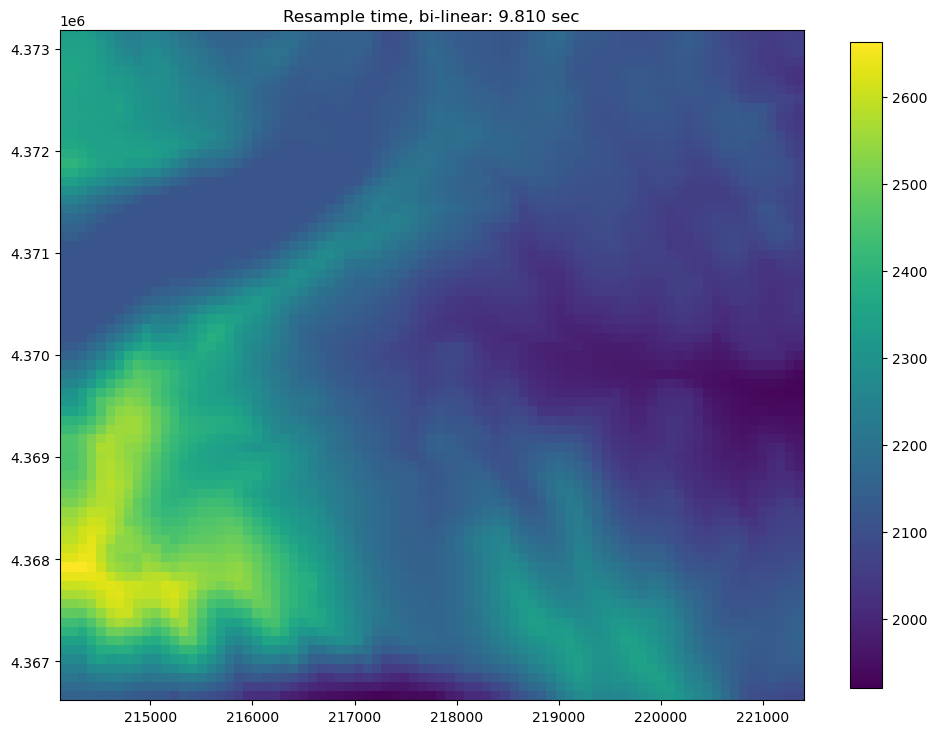
[11]:
t0 = time.time()
dem_data = rio.resample_to_grid(
    ml.modelgrid, band=rio.bands[0], method="linear", extrapolate_edges=True
)
resample_time = time.time() - t0
[12]:
# now to visualize using flopy and matplotlib
fig = plt.figure(figsize=(12, 12))
ax = fig.add_subplot(1, 1, 1, aspect="equal")

pmv = flopy.plot.PlotMapView(modelgrid=ml.modelgrid, ax=ax)
ax = pmv.plot_array(
    dem_data, masked_values=rio.nodatavals, vmin=vmin, vmax=vmax
)
plt.title(f"Resample time, bi-linear: {resample_time:.3f} sec")
plt.colorbar(ax, shrink=0.7)
[12]:
<matplotlib.colorbar.Colorbar at 0x7f99b2965820>
[13]:
t0 = time.time()
dem_data = rio.resample_to_grid(
    ml.modelgrid, band=rio.bands[0], method="cubic", extrapolate_edges=True
)
resample_time = time.time() - t0
[14]:
# now to visualize using flopy and matplotlib
fig = plt.figure(figsize=(12, 12))
ax = fig.add_subplot(1, 1, 1, aspect="equal")

pmv = flopy.plot.PlotMapView(modelgrid=ml.modelgrid, ax=ax)
ax = pmv.plot_array(
    dem_data, masked_values=rio.nodatavals, vmin=vmin, vmax=vmax
)
plt.title(f"Resample time, bi-cubic: {resample_time:.3f} sec")
plt.colorbar(ax, shrink=0.7)
[14]:
<matplotlib.colorbar.Colorbar at 0x7f99a0fa9820>

[15]:
t0 = time.time()
dem_data = rio.resample_to_grid(
    ml.modelgrid,
    band=rio.bands[0],
    method="median",
    extrapolate_edges=True,
)
resample_time = time.time() - t0
[16]:
# now to visualize using flopy and matplotlib
fig = plt.figure(figsize=(12, 12))
ax = fig.add_subplot(1, 1, 1, aspect="equal")

pmv = flopy.plot.PlotMapView(modelgrid=ml.modelgrid, ax=ax)
ax = pmv.plot_array(
    dem_data, masked_values=rio.nodatavals, vmin=vmin, vmax=vmax
)
plt.title(f"Resample time, median: {resample_time:.3f} sec")
plt.colorbar(ax, shrink=0.7)
[16]:
<matplotlib.colorbar.Colorbar at 0x7f99a0f1c6e0>

Vertex and Unstructured grid example
The user can also use either a vertex grid or an unstructured grid and resample raster data to it using the same resample_to_grid() method
Here is an example of building a triangular mesh and creating an unstructured grid instance to use for Raster resampling
[17]:
from flopy.utils.triangle import Triangle

maximum_area = 30000.0  # 30000.

extent = rio.bounds
domainpoly = [
    (extent[0], extent[2]),
    (extent[1], extent[2]),
    (extent[1], extent[3]),
    (extent[0], extent[3]),
]

tri = Triangle(maximum_area=maximum_area, angle=30, model_ws=workspace)

tri.add_polygon(domainpoly)
tri.build(verbose=False)
xc, yc = tri.get_xcyc().T
verts = [[iv, x, y] for iv, (x, y) in enumerate(tri.verts)]
iverts = tri.iverts
ncpl = np.array([len(iverts)])

mg_unstruct = flopy.discretization.UnstructuredGrid(
    vertices=verts, iverts=iverts, ncpl=ncpl, xcenters=xc, ycenters=yc
)
[18]:
# now to visualize using matplotlib
fig = plt.figure(figsize=(12, 12))
ax = fig.add_subplot(1, 1, 1, aspect="equal")

pmv = flopy.plot.PlotMapView(modelgrid=mg_unstruct, ax=ax)
pmv.plot_grid()
[18]:
<matplotlib.collections.LineCollection at 0x7f99b2925d00>

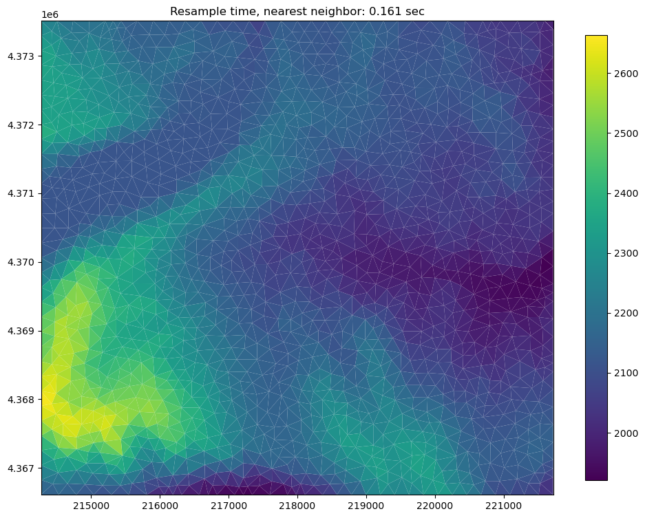
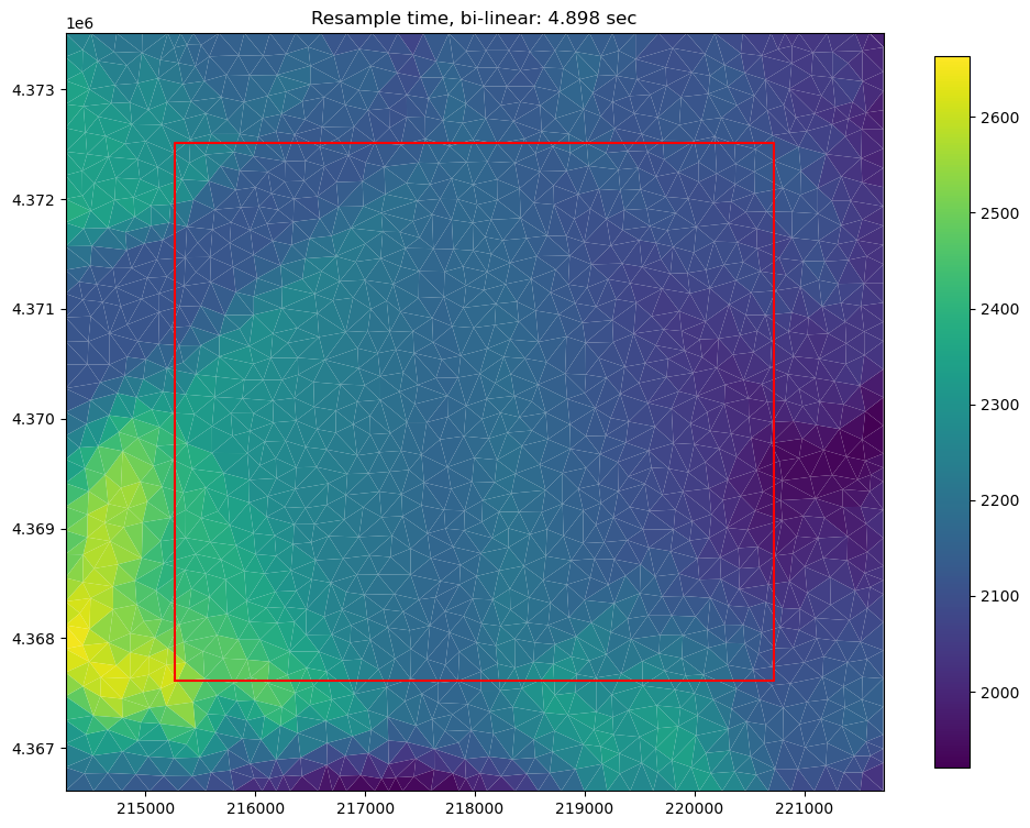
Once a grid object is created, the raster can be resampled to the grid using the same resample_to_grid() method as the structured grid example
[19]:
t0 = time.time()
dem_data = rio.resample_to_grid(
    mg_unstruct, band=rio.bands[0], method="nearest"
)

resample_time = time.time() - t0
[20]:
# now to visualize using flopy and matplotlib
fig = plt.figure(figsize=(12, 12))
ax = fig.add_subplot(1, 1, 1, aspect="equal")

pmv = flopy.plot.PlotMapView(modelgrid=mg_unstruct, ax=ax)
ax = pmv.plot_array(
    dem_data,
    masked_values=rio.nodatavals,
    cmap="viridis",
    vmin=vmin,
    vmax=vmax,
)
plt.title(f"Resample time, nearest neighbor: {resample_time:.3f} sec")
plt.colorbar(ax, shrink=0.7)
[20]:
<matplotlib.colorbar.Colorbar at 0x7f99a0bcc4a0>
[21]:
t0 = time.time()
dem_data = rio.resample_to_grid(
    mg_unstruct, band=rio.bands[0], method="linear"
)

resample_time = time.time() - t0
[22]:
# now to visualize using flopy and matplotlib
fig = plt.figure(figsize=(12, 12))
ax = fig.add_subplot(1, 1, 1, aspect="equal")

pmv = flopy.plot.PlotMapView(modelgrid=mg_unstruct, ax=ax)
ax = pmv.plot_array(
    dem_data,
    masked_values=rio.nodatavals,
    cmap="viridis",
    vmin=vmin,
    vmax=vmax,
)
plt.title(f"Resample time, bi-linear: {resample_time:.3f} sec")
plt.colorbar(ax, shrink=0.7)
[22]:
<matplotlib.colorbar.Colorbar at 0x7f99a08879e0>

[23]:
t0 = time.time()
dem_data = rio.resample_to_grid(
    mg_unstruct,
    band=rio.bands[0],
    method="median",
)

resample_time = time.time() - t0
[24]:
# now to visualize using flopy and matplotlib
fig = plt.figure(figsize=(12, 12))
ax = fig.add_subplot(1, 1, 1, aspect="equal")

pmv = flopy.plot.PlotMapView(modelgrid=mg_unstruct, ax=ax)
ax = pmv.plot_array(
    dem_data,
    masked_values=rio.nodatavals,
    cmap="viridis",
    vmin=vmin,
    vmax=vmax,
)
plt.title(f"Resample time, median: {resample_time:.3f} sec")
plt.colorbar(ax, shrink=0.7)
[24]:
<matplotlib.colorbar.Colorbar at 0x7f99a0941d00>
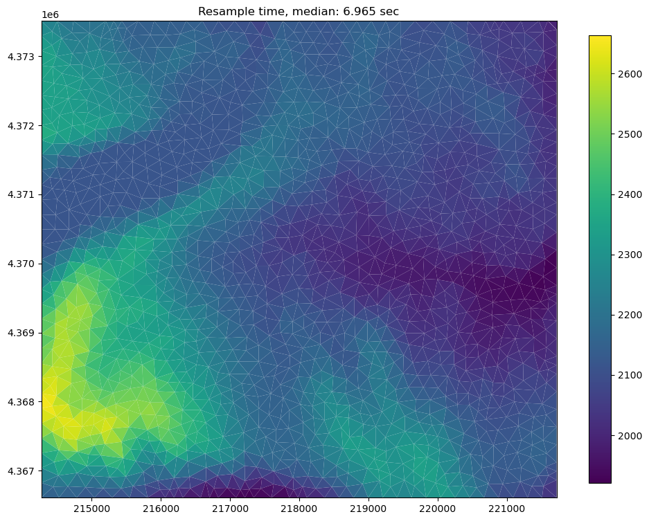
Note: bi-cubic sampling does not work well with triangular meshes and is not recommended for unstructured grids
Sampling points, Cropping, and performing intersections using raster data
The Raster class contains useful methods for sampling single points, cross sections, cropping and performing intersections.
The sample_point() method can be used to sample a single raster value or to sample a cross section
The sample_polygon() method can be used to sample all raster values within an arbitrary polygone
The crop() method allows the user to crop the raster in-place. This method can also be used to perform intersections.
The crop() and sample_polygon() methods apply a modified binary ray casting algorithm for extremely fast intersections. The raster data that’s used for this example contains over 500,000 points. For each intersection every point must be segmented as inside or outside of an arbitratry polygon.
Sampling points or a cross section from the raster
The user can also sample from a points within the raster using the sample_point() method.
This can be used to create simple cross sections of data, such as an elevation profile
[25]:
d = {"easting": [], "northing": [], "elevation": []}

for adj in range(1, 10000, 100):
    easting = xoff + adj
    northing = yoff + adj
    val = rio.sample_point(xoff + adj, yoff + adj, band=1)
    d["easting"].append(easting)
    d["northing"].append(northing)
    d["elevation"].append(val)

df = pd.DataFrame(d)
[26]:
fig = plt.figure(figsize=(12, 12))
ax = fig.add_subplot(1, 1, 1, aspect="equal")

ax.plot(df.easting.values, df.elevation.values, color="saddlebrown")
ax.set_ylabel("Meters elevation (ASL)")
ax.set_xlabel("Easting")
ax.set_title("Elevation profile")

df.head()
[26]:
| easting | northing | elevation | |
|---|---|---|---|
| 0 | 214111 | 4366621 | 2149.143311 |
| 1 | 214211 | 4366721 | 2165.882812 |
| 2 | 214311 | 4366821 | 2198.365234 |
| 3 | 214411 | 4366921 | 2260.733643 |
| 4 | 214511 | 4367021 | 2335.735596 |

Sampling all points within a polygon in the raster
The user can also sample all points within an arbitrary polygon within the raster using the sample_polygon() method.
The sample_polygon() method returns an unordered array of raster values that can be used to perform statical analysis on a chunk of the raster data
[27]:
x0, x1, y0, y1 = rio.bounds

# let's create an a square to use for sampling and cropping
x0 += 1000
y0 += 1000
x1 -= 1000
y1 -= 1000

shape = np.array([(x0, y0), (x0, y1), (x1, y1), (x1, y0), (x0, y0)])
[28]:
fig = plt.figure(figsize=(12, 12))
ax = fig.add_subplot(1, 1, 1, aspect="equal")

ax = rio.plot(ax=ax, vmin=vmin, vmax=vmax)
ax.plot(shape.T[0], shape.T[1], "r-")
plt.colorbar(ax.images[0], shrink=0.7)
[28]:
<matplotlib.colorbar.Colorbar at 0x7f99a08ab350>

[29]:
data = rio.sample_polygon(shape, band=rio.bands[0])

mean = np.mean(data)
dmin = np.min(data)
dmax = np.max(data)
stdv = np.std(data)

s = "Minimum elevation: {:.2f}\nMaximum elevation: {:.2f}\nMean elevation: {:.2f}\nStandard deviation: {:.2f}"
print(s.format(dmin, dmax, mean, stdv))
Minimum elevation: 1942.17
Maximum elevation: 2608.56
Mean elevation: 2151.67
Standard deviation: 113.60
Cropping and resampling to a modelgrid
The crop() method can accept a list or np.array of vertices, a shapely Polygon object, or a GeoJSON dictionary
The crop can also be inverted, using invert=True
[30]:
t0 = time.time()
rio.crop(shape, invert=True)
crop_time = time.time() - t0
[31]:
fig = plt.figure(figsize=(12, 12))
ax = fig.add_subplot(1, 1, 1, aspect="equal")

ax = rio.plot(ax=ax, vmin=vmin, vmax=vmax)
ax.plot(shape.T[0], shape.T[1], "r-")
plt.title(f"Cropping time: {crop_time:.3f} sec")
plt.colorbar(ax.images[0], shrink=0.7)
[31]:
<matplotlib.colorbar.Colorbar at 0x7f99a062aa50>
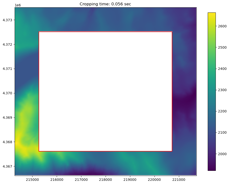
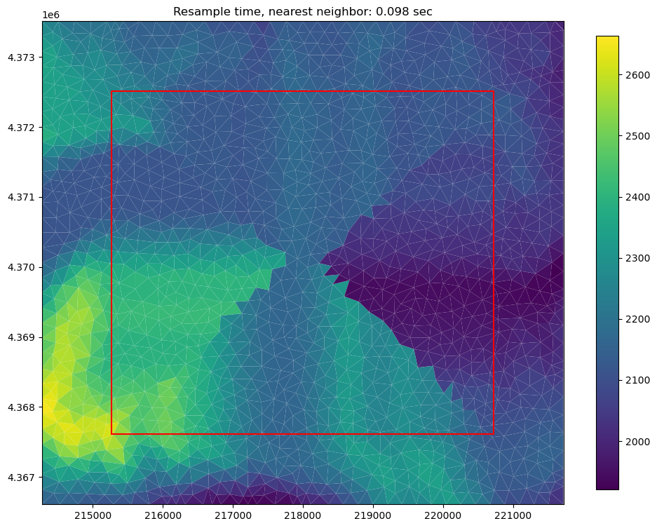
And then this can be re-sampled to a ModelGrid Object
[32]:
t0 = time.time()
dem_data = rio.resample_to_grid(
    mg_unstruct, band=rio.bands[0], method="nearest"
)

resample_time = time.time() - t0
[33]:
# now to visualize using flopy and matplotlib
fig = plt.figure(figsize=(12, 12))
ax = fig.add_subplot(1, 1, 1, aspect="equal")

pmv = flopy.plot.PlotMapView(modelgrid=mg_unstruct, ax=ax)
ax = pmv.plot_array(
    dem_data,
    masked_values=rio.nodatavals,
    cmap="viridis",
    vmin=vmin,
    vmax=vmax,
)
plt.plot(shape.T[0], shape.T[1], "r-")
plt.title(f"Resample time, nearest neighbor: {resample_time:.3f} sec")
plt.colorbar(ax, shrink=0.7)
[33]:
<matplotlib.colorbar.Colorbar at 0x7f99a04fb650>
[34]:
t0 = time.time()
dem_data = rio.resample_to_grid(
    mg_unstruct, band=rio.bands[0], method="linear"
)

resample_time = time.time() - t0
[35]:
# now to visualize using flopy and matplotlib
fig = plt.figure(figsize=(12, 12))
ax = fig.add_subplot(1, 1, 1, aspect="equal")

pmv = flopy.plot.PlotMapView(modelgrid=mg_unstruct, ax=ax)
ax = pmv.plot_array(
    dem_data,
    masked_values=rio.nodatavals,
    cmap="viridis",
    vmin=vmin,
    vmax=vmax,
)
plt.plot(shape.T[0], shape.T[1], "r-")
plt.title(f"Resample time, bi-linear: {resample_time:.3f} sec")
plt.colorbar(ax, shrink=0.7)
[35]:
<matplotlib.colorbar.Colorbar at 0x7f99a03a4f80>
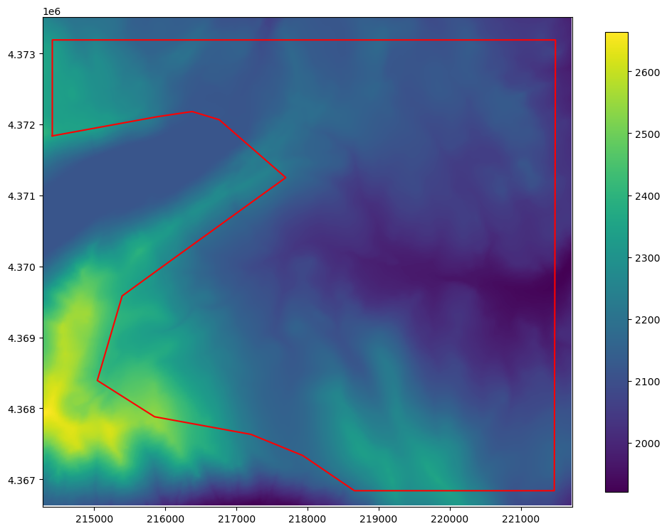
Arbitrary-shaped model boundaries
In the example pyshp and shapely are used to get geometry information and then we create a top array and an ibound array using that geometry information
First let’s reload the raster (since operations are done in-place) and then load our shapefile data
[36]:
rio = Raster.load(os.path.join(raster_ws, raster_name))

shp_name = os.path.join(raster_ws, "model_boundary.shp")

# read in the shapefile
sf = shapefile.Reader(shp_name)
shapes = sf.shapes()
[37]:
fig = plt.figure(figsize=(12, 12))
ax = fig.add_subplot(1, 1, 1, aspect="equal")

ax = rio.plot(ax=ax, vmin=vmin, vmax=vmax)

# plot the shapes for visualization
for shp in shapes:
    shp = np.array(shp.points).T
    plt.plot(shp[0], shp[1], "r-")
plt.colorbar(ax.images[0], shrink=0.7)
[37]:
<matplotlib.colorbar.Colorbar at 0x7f99a02c0ad0>
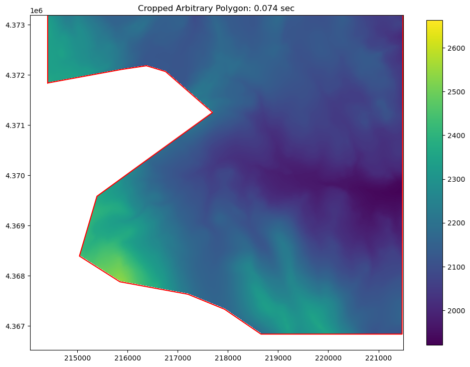
Now we can apply an intersection using the point data directly from the shapefile class
[38]:
polygon = shapes[0].points

t0 = time.time()
rio.crop(polygon)
crop_time = time.time() - t0
[39]:
fig = plt.figure(figsize=(12, 12))
ax = fig.add_subplot(1, 1, 1, aspect="equal")

ax = rio.plot(ax=ax, vmin=vmin, vmax=vmax)

shape = np.array(polygon).T
plt.plot(shape[0], shape[1], "r-")
plt.title(f"Cropped Arbitrary Polygon: {crop_time:.3f} sec")
plt.colorbar(ax.images[0], shrink=0.7)
[39]:
<matplotlib.colorbar.Colorbar at 0x7f99b2bc72f0>
Now the data can be re-sampled to the modelgrid
[40]:
top = rio.resample_to_grid(mg_unstruct, band=rio.bands[0], method="linear")

# apply a "realistic" nodataval to top cells outside the model domain
for val in rio.nodatavals:
    top[top == val] = 3500

# create an ibound array
ibound = np.ones(top.shape, dtype=int)
ibound[top == 3500] = 0
[41]:
# now to visualize using flopy and matplotlib
fig = plt.figure(figsize=(12, 12))
ax = fig.add_subplot(1, 1, 1, aspect="equal")

pmv = flopy.plot.PlotMapView(modelgrid=mg_unstruct, ax=ax)
ax = pmv.plot_array(
    top,
    masked_values=[
        3500,
    ],
    cmap="viridis",
    vmin=vmin,
    vmax=vmax,
)
ib = pmv.plot_ibound(ibound)
pmv.plot_grid(linewidth=0.3)
plt.plot(shape[0], shape[1], "r-")
plt.title(
    "Model top and ibound arrays created using bi-linear raster resampling"
)
plt.colorbar(ax, shrink=0.7)
[41]:
<matplotlib.colorbar.Colorbar at 0x7f99a0f05640>
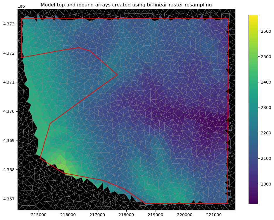
The ibound array and the top array can be used to build or edit the BAS and DIS file objects in FloPy
Raster re-projection
The Raster class has a built in to_crs() method that allows for raster reprojection. The to_crs() method has two possible parameters that can be used to define reprojection and one additional parameter for in place reprojection:
crs: the crs parameter can take many different formats of coordinate refence systems (WKT string, epsg code, pyproj.CRS, rasterio.CRS, proj4 string, epsg string, etc…)epsg: integer epsg numberinplace: bool, default False creates a new raster object, True modifies the existing Raster object
Here’s example usage:
[42]:
cur_crs = rio.crs
print(cur_crs)
print(rio.transform)
EPSG:26911
| 10.00, 0.00, 214410.00|
| 0.00,-10.00, 4373190.00|
| 0.00, 0.00, 1.00|
[43]:
rio_reproj = rio.to_crs(crs="EPSG:4326")  # WGS84 dec. lat lon
print(rio_reproj.crs)
print(rio_reproj.transform)
EPSG:4326
| 0.00, 0.00,-120.32|
| 0.00,-0.00, 39.46|
| 0.00, 0.00, 1.00|
Reproject as an inplace operation
[44]:
rio.to_crs(epsg=4326, inplace=True)
print(rio.crs)
print(rio.transform)
EPSG:4326
| 0.00, 0.00,-120.32|
| 0.00,-0.00, 39.46|
| 0.00, 0.00, 1.00|
Future development
Potential features that draw on this functionality could include: + intersection with multiple polygons + flow accumulation to develop SFR networks + streambed topology from raster layers + intersection with layers of derived parameters based on multiple raster bands
[45]:
try:
    # ignore PermissionError on Windows
    temp_dir.cleanup()
except:
    pass