This page was generated from mf6_parallel_model_splitting_example.py. It's also available as a notebook.

Model splitting for parallel and serial MODFLOW 6

The model splitting functionality for MODFLOW 6 is shown in this notebook. Model splitting via the Mf6Splitter() class can be performed on groundwater flow models as well as combined groundwater flow and transport models. The Mf6Splitter() class maps a model’s connectivity and then builds new models, with exchanges and movers between the new models, based on a user defined array of model numbers.

The Mf6Splitter() class supports Structured, Vertex, and Unstructured Grid models.

import sys
from pathlib import Path
from tempfile import TemporaryDirectory

import matplotlib.pyplot as plt
import numpy as np

import flopy
from flopy.mf6.utils import Mf6Splitter
from flopy.plot import styles
from flopy.utils.geometry import LineString, Polygon

sys.path.append("../common")
from notebook_utils import geometries, string2geom

Example 1: splitting a simple structured grid model

This example shows the basics of using the Mf6Splitter() class and applies the method to the Freyberg (1988) model.

simulation_ws = Path("../../examples/data/mf6-freyberg")
sim = flopy.mf6.MFSimulation.load(sim_ws=simulation_ws)

loading simulation...
  loading simulation name file...
  loading tdis package...
  loading model gwf6...
    loading package dis...
    loading package ic...
WARNING: Block "options" is not a valid block name for file type ic.
    loading package oc...
    loading package npf...
    loading package sto...
    loading package chd...
    loading package riv...
    loading package wel...
    loading package rch...
  loading solution package freyberg...

Create a temporary directory for this example and run the Freyberg (1988) model.

temp_dir = TemporaryDirectory()
workspace = Path(temp_dir.name)

sim.set_sim_path(workspace)
sim.write_simulation()
success, buff = sim.run_simulation(silent=True)
assert success

writing simulation...
  writing simulation name file...
  writing simulation tdis package...
  writing solution package freyberg...
  writing model freyberg...
    writing model name file...
    writing package dis...
    writing package ic...
    writing package oc...
    writing package npf...
    writing package sto...
    writing package chd-1...
    writing package riv-1...
    writing package wel-1...
    writing package rch-1...

Visualize the head results and boundary conditions from this model.

gwf = sim.get_model()
head = gwf.output.head().get_alldata()[-1]

fig, ax = plt.subplots(figsize=(5, 7))
pmv = flopy.plot.PlotMapView(gwf, ax=ax)
heads = gwf.output.head().get_alldata()[-1]
heads = np.where(heads == 1e30, np.nan, heads)
vmin = np.nanmin(heads)
vmax = np.nanmax(heads)
pc = pmv.plot_array(heads, vmin=vmin, vmax=vmax)
pmv.plot_bc("WEL")
pmv.plot_bc("RIV", color="c")
pmv.plot_bc("CHD")
pmv.plot_grid()
pmv.plot_ibound()
plt.colorbar(pc)

<matplotlib.colorbar.Colorbar at 0x7f885a8976b0>

Creating an array that defines the new models

In order to split models, the model domain must be discretized using unique model numbers. Any number of models can be created, however all of the cells within each model must be contiguous.

The Mf6Splitter() class accept arrays that are equal in size to the number of cells per layer (StructuredGrid and VertexGrid) or the number of model nodes (UnstructuredGrid).

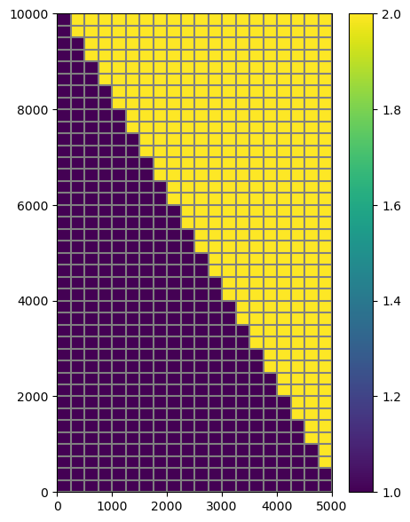
In this example, the model is split diagonally into two model domains.

modelgrid = gwf.modelgrid

array = np.ones((modelgrid.nrow, modelgrid.ncol), dtype=int)
ncol = 1
for row in range(modelgrid.nrow):
    if row != 0 and row % 2 == 0:
        ncol += 1
    array[row, ncol:] = 2

Plot the two domains that the model will be split into

fig, ax = plt.subplots(figsize=(5, 7))
pmv = flopy.plot.PlotMapView(gwf, ax=ax)
pc = pmv.plot_array(array)
lc = pmv.plot_grid()
plt.colorbar(pc)
plt.show()

Splitting the model using Mf6Splitter()

The Mf6Splitter() class accepts one required parameter and one optional parameter. These parameters are: - sim: A flopy.mf6.MFSimulation object - modelname: optional, the name of the model being split. If omitted Mf6Splitter grabs the first groundwater flow model listed in the simulation

mfsplit = Mf6Splitter(sim)

The model splitting is then performed by calling the split_model() function. split_model() accepts an array that is either the same size as the number of cells per layer (StructuredGrid and VertexGrid) model or the number of nodes in the model (UnstructuredGrid).

This function returns a new MFSimulation object that contains the split models and exchanges between them

new_sim = mfsplit.split_model(array)

# now to write and run the simulation
new_sim.set_sim_path(workspace / "split_model")
new_sim.write_simulation()
success, buff = new_sim.run_simulation(silent=True)
assert success

writing simulation...
  writing simulation name file...
  writing simulation tdis package...
  writing solution package ims_-1...
  writing package sim_1_2.gwfgwf...
  writing model freyberg_1...
    writing model name file...
    writing package dis...
    writing package ic...
    writing package oc...
    writing package npf...
    writing package sto...
    writing package chd-1...
    writing package riv-1...
    writing package wel-1...
    writing package rch-1...
  writing model freyberg_2...
    writing model name file...
    writing package dis...
    writing package ic...
    writing package oc...
    writing package npf...
    writing package sto...
    writing package riv-1...
    writing package wel-1...
    writing package rch-1...

Visualize and reassemble model output

Both models are visualized side by side

# visualizing both models side by side
ml0 = new_sim.get_model("freyberg_1")
ml1 = new_sim.get_model("freyberg_2")

heads0 = ml0.output.head().get_alldata()[-1]
heads1 = ml1.output.head().get_alldata()[-1]

fig, (ax0, ax1) = plt.subplots(1, 2, figsize=(12, 7))
pmv = flopy.plot.PlotMapView(ml0, ax=ax0)
pmv.plot_array(heads0, vmin=vmin, vmax=vmax)
pmv.plot_ibound()
pmv.plot_grid()
pmv.plot_bc("WEL")
pmv.plot_bc("RIV", color="c")
pmv.plot_bc("CHD")
ax0.set_title("Model 0")

pmv = flopy.plot.PlotMapView(ml1, ax=ax1)
pc = pmv.plot_array(heads1, vmin=vmin, vmax=vmax)
pmv.plot_ibound()
pmv.plot_bc("WEL")
pmv.plot_bc("RIV", color="c")
pmv.plot_grid()
ax1.set_title("Model 1")

fig.subplots_adjust(right=0.8)
cbar_ax = fig.add_axes([0.85, 0.15, 0.05, 0.7])
cbar = fig.colorbar(pc, cax=cbar_ax, label="Hydraulic heads")

Array based model output can be assembled into the original model’s shape by using the reconstruct_array() method

reconstruct_array accepts a dictionary of array data. This data is assembled as {model_number: array_from_model}.

array_dict = {1: heads0, 2: heads1}

new_head_array = mfsplit.reconstruct_array(array_dict)

Recarray based model inputs and outputs can also be assembled into the original model’s shape by using the reconstruct_recarray() method

The code below demonstratess how to join the input recarrays for the WEL, RIV, and CHD package and plot them as boundary condition arrays.

models = [ml0, ml1]

pkgs = ["wel", "riv", "chd"]
d = {}
for pkg in pkgs:
    rarrays = {}
    for ix, model in enumerate(models):
        pak = model.get_package(pkg)
        try:
            rarrays[ix + 1] = pak.stress_period_data.data[0]
        except (TypeError, AttributeError):
            pass
    recarray = mfsplit.reconstruct_recarray(rarrays)
    if pkg == "riv":
        color = "c"
        bc_array, kwargs = mfsplit.recarray_bc_array(recarray, color="c")
    else:
        bc_array, kwargs = mfsplit.recarray_bc_array(recarray, pkgtype=pkg)
    d[pkg] = {"bc_array": bc_array, "kwargs": kwargs}

fig, ax = plt.subplots(figsize=(5, 7))
pmv = flopy.plot.PlotMapView(gwf, ax=ax)
pc = pmv.plot_array(new_head_array, vmin=vmin, vmax=vmax)
pmv.plot_ibound()
pmv.plot_grid()
pmv.plot_array(d["wel"]["bc_array"], **d["wel"]["kwargs"])
pmv.plot_array(d["riv"]["bc_array"], **d["riv"]["kwargs"])
pmv.plot_array(d["chd"]["bc_array"], **d["chd"]["kwargs"])
plt.colorbar(pc)
plt.show()

Example 2: a more comprehensive example with the watershed model from Hughes and others 2023

In this example, a basin model is created and is split into many models. From Hughes, Joseph D., Langevin, Christian D., Paulinski, Scott R., Larsen, Joshua D., and Brakenhoff, David, 2023, FloPy Workflows for Creating Structured and Unstructured MODFLOW Models: Groundwater, https://doi.org/10.1111/gwat.13327

Create the model

Load an ASCII raster file

ascii_file = Path("../../examples/data/geospatial/fine_topo.asc")

fine_topo = flopy.utils.Raster.load(ascii_file)
fine_topo.plot()

<Axes: >

Lx = 180000
Ly = 100000
extent = (0, Lx, 0, Ly)
levels = np.arange(10, 110, 10)
vmin, vmax = 0.0, 100.0

temp_dir = TemporaryDirectory()
workspace = Path(temp_dir.name)

boundary_polygon = string2geom(geometries["boundary"])
boundary_polygon.append(boundary_polygon[0])
bp = np.array(boundary_polygon)

# define stream segment locations
segs = [string2geom(geometries[f"streamseg{i}"]) for i in range(1, 5)]

Plot the model boundary and the individual stream segments for the RIV package

fig = plt.figure(figsize=(8, 8))
ax = fig.add_subplot()
ax.set_aspect("equal")
riv_colors = ("blue", "cyan", "green", "orange", "red")
ax.plot(bp[:, 0], bp[:, 1], "ro-")
for idx, seg in enumerate(segs):
    sa = np.array(seg)
    ax.plot(sa[:, 0], sa[:, 1], color=riv_colors[idx], lw=0.75, marker="o")

Create a MODFLOW model grid

dx = dy = 5000
dv0 = 5.0
nlay = 1
nrow = int(Ly / dy) + 1
ncol = int(Lx / dx) + 1
delr = np.array(ncol * [dx])
delc = np.array(nrow * [dy])
top = np.ones((nrow, ncol)) * 1000.0
botm = np.ones((nlay, nrow, ncol)) * -100.0
modelgrid = flopy.discretization.StructuredGrid(
    nlay=nlay, delr=delr, delc=delc, xoff=0, yoff=0, top=top, botm=botm
)

Crop the raster, resample it for the top elevation, and create an ibound array

new_top = fine_topo.resample_to_grid(
    modelgrid, band=fine_topo.bands[0], method="min", extrapolate_edges=True
)

# calculate and set idomain
ix = flopy.utils.GridIntersect(modelgrid, method="vertex", rtree=True)
result = ix.intersect(Polygon(boundary_polygon))
idxs = tuple(zip(*result.cellids))
idomain = np.zeros((nrow, ncol), dtype=int)
idomain[idxs] = 1

# set this idomain and top to the modelgrid
modelgrid._idomain = idomain
modelgrid._top = new_top

Intersect the stream segments with the modelgrid

ixs = flopy.utils.GridIntersect(modelgrid, method="structured")
cellids = []
for seg in segs:
    v = ixs.intersect(LineString(seg), sort_by_cellid=True)
    cellids += v["cellids"].tolist()
intersection_rg = np.zeros(modelgrid.shape[1:])
for loc in cellids:
    intersection_rg[loc] = 1

with styles.USGSMap():
    fig, ax = plt.subplots(figsize=(8, 8))
    pmv = flopy.plot.PlotMapView(modelgrid=modelgrid)
    ax.set_aspect("equal")
    pmv.plot_array(modelgrid.top)
    pmv.plot_array(
        intersection_rg,
        masked_values=[
            0,
        ],
        alpha=0.2,
        cmap="Reds_r",
    )
    pmv.plot_inactive()
    ax.plot(bp[:, 0], bp[:, 1], "r-")
    for seg in segs:
        sa = np.array(seg)
        ax.plot(sa[:, 0], sa[:, 1], "b-")

Calculate drain conductance, set simulation options, and begin building model arrays

# Set number of model layers to 2
nlay = 2

# intersect stream segs to simulate as drains
ixs = flopy.utils.GridIntersect(modelgrid, method="structured")
drn_cellids = []
drn_lengths = []
for seg in segs:
    v = ixs.intersect(LineString(seg), sort_by_cellid=True)
    drn_cellids += v["cellids"].tolist()
    drn_lengths += v["lengths"].tolist()

leakance = 1.0 / (0.5 * dv0)  # kv / b
drn_data = []
for (r, c), length in zip(drn_cellids, drn_lengths):
    x = modelgrid.xcellcenters[r, c]
    width = 5.0 + (14.0 / Lx) * (Lx - x)
    conductance = leakance * length * width
    drn_data.append((0, r, c, modelgrid.top[r, c], conductance))
drn_data[:10]

[(0, 12, 36, 3.6404473781585693, 9622.185546471488),
 (0, 12, 35, 1.111111044883728, 10478.844160380193),
 (0, 12, 34, 3.8888888359069824, 11731.97414523631),
 (0, 12, 33, 6.666666507720947, 12346.648887868123),
 (0, 12, 32, 9.44444465637207, 6006.996161832478),
 (0, 11, 32, 10.555556297302246, 6942.175535223257),
 (0, 11, 31, 12.222222328186035, 13534.73438485134),
 (0, 11, 30, 15.0, 14284.510735821312),
 (0, 11, 29, 17.77777862548828, 13441.64541297737),
 (0, 12, 29, 20.0, 1699.7820641189026)]

# groundwater discharge to surface
idomain = modelgrid.idomain.copy()
index = tuple(zip(*drn_cellids))
idomain[index] = -1

gw_discharge_data = []
for r in range(nrow):
    for c in range(ncol):
        if idomain[r, c] < 1:
            continue
        conductance = leakance * dx * dy
        gw_discharge_data.append(
            (0, r, c, modelgrid.top[r, c] - 0.5, conductance, 1.0)
        )
gw_discharge_data[:10]

[(0, 1, 7, 99.99099731445312, 10000000.0, 1.0),
 (0, 1, 8, 98.9864730834961, 10000000.0, 1.0),
 (0, 1, 9, 97.68162536621094, 10000000.0, 1.0),
 (0, 1, 10, 96.02616882324219, 10000000.0, 1.0),
 (0, 1, 11, 93.93696594238281, 10000000.0, 1.0),
 (0, 1, 12, 91.06060028076172, 10000000.0, 1.0),
 (0, 1, 13, 87.65284729003906, 10000000.0, 1.0),
 (0, 1, 14, 86.53125, 10000000.0, 1.0),
 (0, 2, 5, 100.72657012939453, 10000000.0, 1.0),
 (0, 2, 6, 100.33457946777344, 10000000.0, 1.0)]

botm = np.zeros((nlay, nrow, ncol))
botm[0] = modelgrid.top - dv0
for ix in range(1, nlay):
    dv0 *= 1.5
    botm[ix] = botm[ix - 1] - dv0

idomain = np.zeros((nlay, nrow, ncol), dtype=int)
idomain[:] = modelgrid.idomain

strt = np.zeros((nlay, nrow, ncol))
strt[:] = modelgrid.top

Create the watershed model using Flopy

temp_dir = TemporaryDirectory()
workspace = Path(temp_dir.name) / "basin"

sim = flopy.mf6.MFSimulation(
    sim_name="basin",
    sim_ws=workspace,
    exe_name="mf6",
)

tdis = flopy.mf6.ModflowTdis(sim)
ims = flopy.mf6.ModflowIms(
    sim,
    complexity="simple",
    print_option="SUMMARY",
    linear_acceleration="bicgstab",
    outer_maximum=1000,
    inner_maximum=100,
    outer_dvclose=1e-5,
    inner_dvclose=1e-6,
)
gwf = flopy.mf6.ModflowGwf(
    sim,
    save_flows=True,
    newtonoptions="NEWTON UNDER_RELAXATION",
)

dis = flopy.mf6.ModflowGwfdis(
    gwf,
    nlay=nlay,
    nrow=nrow,
    ncol=ncol,
    delr=dx,
    delc=dy,
    idomain=idomain,
    top=modelgrid.top,
    botm=botm,
    xorigin=0.0,
    yorigin=0.0,
)

ic = flopy.mf6.ModflowGwfic(gwf, strt=strt)
npf = flopy.mf6.ModflowGwfnpf(
    gwf,
    save_specific_discharge=True,
    icelltype=1,
    k=1.0,
)
sto = flopy.mf6.ModflowGwfsto(
    gwf,
    iconvert=1,
    ss=1e-5,
    sy=0.2,
    steady_state=True,
)
rch = flopy.mf6.ModflowGwfrcha(
    gwf,
    recharge=0.000001,
)
drn = flopy.mf6.ModflowGwfdrn(
    gwf,
    stress_period_data=drn_data,
    pname="river",
)
drn_gwd = flopy.mf6.ModflowGwfdrn(
    gwf,
    auxiliary=["depth"],
    auxdepthname="depth",
    stress_period_data=gw_discharge_data,
    pname="gwd",
)
oc = flopy.mf6.ModflowGwfoc(
    gwf,
    head_filerecord=f"{gwf.name}.hds",
    budget_filerecord=f"{gwf.name}.cbc",
    saverecord=[("HEAD", "ALL"), ("BUDGET", "ALL")],
    printrecord=[("BUDGET", "ALL")],
)

sim.write_simulation()
success, buff = sim.run_simulation(silent=True)
assert success

writing simulation...
  writing simulation name file...
  writing simulation tdis package...
  writing solution package ims_-1...
  writing model model...
    writing model name file...
    writing package dis...
    writing package ic...
    writing package npf...
    writing package sto...
    writing package rcha_0...
    writing package river...
INFORMATION: maxbound in ('gwf6', 'drn', 'dimensions') changed to 88 based on size of stress_period_data
    writing package gwd...
INFORMATION: maxbound in ('gwf6', 'drn', 'dimensions') changed to 470 based on size of stress_period_data
    writing package oc...

Plot the model results

water_table = flopy.utils.postprocessing.get_water_table(
    gwf.output.head().get_data()
)
heads = gwf.output.head().get_data()
hmin, hmax = water_table.min(), water_table.max()
contours = np.arange(0, 100, 10)
hmin, hmax

(1.1351828297118696, 105.96803703036794)

with styles.USGSMap():
    fig = plt.figure(figsize=(10, 8))
    ax = fig.add_subplot()
    ax.set_xlim(0, Lx)
    ax.set_ylim(0, Ly)
    ax.set_aspect("equal")
    pmv = flopy.plot.PlotMapView(modelgrid=gwf.modelgrid, ax=ax)
    h = pmv.plot_array(heads, vmin=hmin, vmax=hmax)
    c = pmv.contour_array(
        water_table,
        levels=contours,
        colors="white",
        linewidths=0.75,
        linestyles=":",
    )
    plt.clabel(c, fontsize=8)
    pmv.plot_inactive()
    plt.colorbar(h, ax=ax, shrink=0.5)

    ax.plot(bp[:, 0], bp[:, 1], "r-")
    for seg in segs:
        sa = np.array(seg)
        ax.plot(sa[:, 0], sa[:, 1], "b-")

Split the watershed model

Build a splitting array and split this model into many models for parallel modflow runs

nrow_blocks, ncol_blocks = 2, 4
row_inc, col_inc = int(nrow / nrow_blocks), int(ncol / ncol_blocks)
row_inc, col_inc

(10, 9)

icnt = 0
row_blocks = [icnt]
for i in range(nrow_blocks):
    icnt += row_inc
    row_blocks.append(icnt)
if row_blocks[-1] < nrow:
    row_blocks[-1] = nrow
row_blocks

[0, 10, 21]

icnt = 0
col_blocks = [icnt]
for i in range(ncol_blocks):
    icnt += col_inc
    col_blocks.append(icnt)
if col_blocks[-1] < ncol:
    col_blocks[-1] = ncol
col_blocks

[0, 9, 18, 27, 37]

mask = np.zeros((nrow, ncol), dtype=int)

# create masking array
ival = 1
model_row_col_offset = {}
for idx in range(len(row_blocks) - 1):
    for jdx in range(len(col_blocks) - 1):
        mask[
            row_blocks[idx] : row_blocks[idx + 1],
            col_blocks[jdx] : col_blocks[jdx + 1],
        ] = ival
        model_row_col_offset[ival - 1] = (row_blocks[idx], col_blocks[jdx])
        # increment model number
        ival += 1

plt.imshow(mask)

<matplotlib.image.AxesImage at 0x7f8840448470>

Now split the model into many models using Mf6Splitter()

mfsplit = Mf6Splitter(sim)
new_sim = mfsplit.split_model(mask)

new_ws = workspace / "split_models"
new_sim.set_sim_path(new_ws)
new_sim.write_simulation()
success, buff = new_sim.run_simulation(silent=True)
assert success

writing simulation...
  writing simulation name file...
  writing simulation tdis package...
  writing solution package ims_-1...
  writing package sim_1_2.gwfgwf...
  writing package sim_1_5.gwfgwf...
  writing package sim_2_3.gwfgwf...
  writing package sim_2_6.gwfgwf...
  writing package sim_3_4.gwfgwf...
  writing package sim_3_7.gwfgwf...
  writing package sim_4_8.gwfgwf...
  writing package sim_5_6.gwfgwf...
  writing package sim_6_7.gwfgwf...
  writing package sim_7_8.gwfgwf...
  writing model model_1...
    writing model name file...
    writing package dis...
    writing package ic...
    writing package npf...
    writing package sto...
    writing package rcha_0...
    writing package river...
    writing package gwd...
    writing package oc...
  writing model model_2...
    writing model name file...
    writing package dis...
    writing package ic...
    writing package npf...
    writing package sto...
    writing package rcha_0...
    writing package river...
    writing package gwd...
    writing package oc...
  writing model model_3...
    writing model name file...
    writing package dis...
    writing package ic...
    writing package npf...
    writing package sto...
    writing package rcha_0...
    writing package river...
    writing package gwd...
    writing package oc...
  writing model model_4...
    writing model name file...
    writing package dis...
    writing package ic...
    writing package npf...
    writing package sto...
    writing package rcha_0...
    writing package gwd...
    writing package oc...
  writing model model_5...
    writing model name file...
    writing package dis...
    writing package ic...
    writing package npf...
    writing package sto...
    writing package rcha_0...
    writing package river...
    writing package gwd...
    writing package oc...
  writing model model_6...
    writing model name file...
    writing package dis...
    writing package ic...
    writing package npf...
    writing package sto...
    writing package rcha_0...
    writing package river...
    writing package gwd...
    writing package oc...
  writing model model_7...
    writing model name file...
    writing package dis...
    writing package ic...
    writing package npf...
    writing package sto...
    writing package rcha_0...
    writing package river...
    writing package gwd...
    writing package oc...
  writing model model_8...
    writing model name file...
    writing package dis...
    writing package ic...
    writing package npf...
    writing package sto...
    writing package rcha_0...
    writing package river...
    writing package gwd...
    writing package oc...

Reassemble the heads to the original model shape for plotting

Create a dictionary of model number : heads and use the reconstruct_array() method to get a numpy array that is the original shape of the unsplit model.

model_names = list(new_sim.model_names)
head_dict = {}
for modelname in model_names:
    mnum = int(modelname.split("_")[-1])
    head = new_sim.get_model(modelname).output.head().get_alldata()[-1]
    head_dict[mnum] = head

ra_heads = mfsplit.reconstruct_array(head_dict)
ra_watertable = flopy.utils.postprocessing.get_water_table(ra_heads)

with styles.USGSMap():
    fig, axs = plt.subplots(nrows=3, figsize=(8, 12))
    diff = ra_heads - heads
    hv = [ra_heads, heads, diff]
    titles = ["Multiple models", "Single model", "Multiple - single"]
    for idx, ax in enumerate(axs):
        ax.set_aspect("equal")
        ax.set_title(titles[idx])

        if idx < 2:
            levels = contours
            vmin = hmin
            vmax = hmax
        else:
            levels = None
            vmin = None
            vmax = None

        pmv = flopy.plot.PlotMapView(modelgrid=gwf.modelgrid, ax=ax, layer=0)
        h = pmv.plot_array(hv[idx], vmin=vmin, vmax=vmax)
        if levels is not None:
            c = pmv.contour_array(
                hv[idx],
                levels=levels,
                colors="white",
                linewidths=0.75,
                linestyles=":",
            )
            plt.clabel(c, fontsize=8)
        pmv.plot_inactive()
        plt.colorbar(h, ax=ax, shrink=0.5)

        ax.plot(bp[:, 0], bp[:, 1], "r-")
        for seg in segs:
            sa = np.array(seg)
            ax.plot(sa[:, 0], sa[:, 1], "b-")

Example 3: create an optimized splitting mask for a model

In the previous examples, the watershed model splitting mask was defined by the user. Mf6Splitter also has a method called optimize_splitting_mask that creates a mask based on the number of models the user would like to generate.

The optimize_splitting_mask() method generates a vertex weighted adjacency graph, based on the number active and inactive nodes in all layers of the model. This adjacency graph is then provided to pymetis which does the work for us and returns a membership array for each node.

# Split the watershed model into many models
mfsplit = Mf6Splitter(sim)
split_array = mfsplit.optimize_splitting_mask(nparts=8)

with styles.USGSMap():
    fig, ax = plt.subplots(figsize=(12, 8))
    pmv = flopy.plot.PlotMapView(gwf, ax=ax)
    pmv.plot_array(split_array)
    pmv.plot_inactive()
    pmv.plot_grid()

new_sim = mfsplit.split_model(split_array)

temp_dir = TemporaryDirectory()
workspace = Path("temp")

new_ws = workspace / "opt_split_models"
new_sim.set_sim_path(new_ws)
new_sim.write_simulation()
success, buff = new_sim.run_simulation(silent=True)
assert success

writing simulation...
  writing simulation name file...
  writing simulation tdis package...
  writing solution package ims_-1...
  writing package sim_0_1.gwfgwf...
  writing package sim_0_2.gwfgwf...
  writing package sim_0_4.gwfgwf...
  writing package sim_0_5.gwfgwf...
  writing package sim_1_3.gwfgwf...
  writing package sim_2_3.gwfgwf...
  writing package sim_2_5.gwfgwf...
  writing package sim_2_6.gwfgwf...
  writing package sim_4_5.gwfgwf...
  writing package sim_4_7.gwfgwf...
  writing package sim_5_6.gwfgwf...
  writing package sim_5_7.gwfgwf...
  writing package sim_6_7.gwfgwf...
  writing model model_0...
    writing model name file...
    writing package dis...
    writing package ic...
    writing package npf...
    writing package sto...
    writing package rcha_0...
    writing package river...
    writing package gwd...
    writing package oc...
  writing model model_1...
    writing model name file...
    writing package dis...
    writing package ic...
    writing package npf...
    writing package sto...
    writing package rcha_0...
    writing package river...
    writing package gwd...
    writing package oc...
  writing model model_2...
    writing model name file...
    writing package dis...
    writing package ic...
    writing package npf...
    writing package sto...
    writing package rcha_0...
    writing package river...
    writing package gwd...
    writing package oc...
  writing model model_3...
    writing model name file...
    writing package dis...
    writing package ic...
    writing package npf...
    writing package sto...
    writing package rcha_0...
    writing package river...
    writing package gwd...
    writing package oc...
  writing model model_4...
    writing model name file...
    writing package dis...
    writing package ic...
    writing package npf...
    writing package sto...
    writing package rcha_0...
    writing package river...
    writing package gwd...
    writing package oc...
  writing model model_5...
    writing model name file...
    writing package dis...
    writing package ic...
    writing package npf...
    writing package sto...
    writing package rcha_0...
    writing package river...
    writing package gwd...
    writing package oc...
  writing model model_6...
    writing model name file...
    writing package dis...
    writing package ic...
    writing package npf...
    writing package sto...
    writing package rcha_0...
    writing package river...
    writing package gwd...
    writing package oc...
  writing model model_7...
    writing model name file...
    writing package dis...
    writing package ic...
    writing package npf...
    writing package sto...
    writing package rcha_0...
    writing package river...
    writing package gwd...
    writing package oc...

Reassemble the heads and plot results

model_names = list(new_sim.model_names)
head_dict = {}
for modelname in model_names:
    mnum = int(modelname.split("_")[-1])
    head = new_sim.get_model(modelname).output.head().get_alldata()[-1]
    head_dict[mnum] = head

ra_heads = mfsplit.reconstruct_array(head_dict)
ra_watertable = flopy.utils.postprocessing.get_water_table(ra_heads)

with styles.USGSMap():
    fig, axs = plt.subplots(nrows=3, figsize=(8, 12))
    diff = ra_heads - heads
    hv = [ra_heads, heads, diff]
    titles = ["Multiple models", "Single model", "Multiple - single"]
    for idx, ax in enumerate(axs):
        ax.set_aspect("equal")
        ax.set_title(titles[idx])

        if idx < 2:
            levels = contours
            vmin = hmin
            vmax = hmax
        else:
            levels = None
            vmin = None
            vmax = None

        pmv = flopy.plot.PlotMapView(modelgrid=gwf.modelgrid, ax=ax, layer=0)
        h = pmv.plot_array(hv[idx], vmin=vmin, vmax=vmax)
        if levels is not None:
            c = pmv.contour_array(
                hv[idx],
                levels=levels,
                colors="white",
                linewidths=0.75,
                linestyles=":",
            )
            plt.clabel(c, fontsize=8)
        pmv.plot_inactive()
        plt.colorbar(h, ax=ax, shrink=0.5)

        ax.plot(bp[:, 0], bp[:, 1], "r-")
        for seg in segs:
            sa = np.array(seg)
            ax.plot(sa[:, 0], sa[:, 1], "b-")