This page was generated from get_transmissivities_example.py. It's also available as a notebook.

Computing transmissivity-weighted averages

Demonstration of flopy.utils.get_transmissivities method for computing open interval transmissivities (for weighted averages of heads or fluxes) In practice this method might be used to:

• compute vertically-averaged head target values representative of observation wells of varying open intervals (including variability in saturated thickness due to the position of the water table)

• apportion boundary fluxes (e.g. from an analytic element model) among model layers based on transmissivity.

• any other analysis where a distribution of transmissivity by layer is needed for a specified vertical interval of the model.

import sys
from tempfile import TemporaryDirectory

import matplotlib as mpl
import matplotlib.pyplot as plt
import numpy as np

import flopy

print(sys.version)
print(f"numpy version: {np.__version__}")
print(f"matplotlib version: {mpl.__version__}")
print(f"flopy version: {flopy.__version__}")

3.12.2 | packaged by conda-forge | (main, Feb 16 2024, 20:50:58) [GCC 12.3.0]
numpy version: 1.26.4
matplotlib version: 3.8.4
flopy version: 3.7.0.dev0

Make up some open interval tops and bottoms and some heads

• (these could be lists of observation well screen tops and bottoms)

• the heads array contains the simulated head in each model layer, at the location of each observation well (for example, what you would get back from HYDMOD if you had an entry for each layer at the location of each head target).

• make up a model grid with uniform horizontal k of 2.

sctop = [-0.25, 0.5, 1.7, 1.5, 3.0, 2.5]  # screen tops
scbot = [-1.0, -0.5, 1.2, 0.5, 1.5, -0.2]  # screen bottoms
# head in each layer, for 6 head target locations
heads = np.array(
    [
        [1.0, 2.0, 2.05, 3.0, 4.0, 2.5],
        [1.1, 2.1, 2.2, 2.0, 3.5, 3.0],
        [1.2, 2.3, 2.4, 0.6, 3.4, 3.2],
    ]
)
nl, nr = heads.shape
nc = nr
botm = np.ones((nl, nr, nc), dtype=float)
top = np.ones((nr, nc), dtype=float) * 2.1
hk = np.ones((nl, nr, nc), dtype=float) * 2.0
for i in range(nl):
    botm[nl - i - 1, :, :] = i
botm

array([[[2., 2., 2., 2., 2., 2.],
        [2., 2., 2., 2., 2., 2.],
        [2., 2., 2., 2., 2., 2.],
        [2., 2., 2., 2., 2., 2.],
        [2., 2., 2., 2., 2., 2.],
        [2., 2., 2., 2., 2., 2.]],

       [[1., 1., 1., 1., 1., 1.],
        [1., 1., 1., 1., 1., 1.],
        [1., 1., 1., 1., 1., 1.],
        [1., 1., 1., 1., 1., 1.],
        [1., 1., 1., 1., 1., 1.],
        [1., 1., 1., 1., 1., 1.]],

       [[0., 0., 0., 0., 0., 0.],
        [0., 0., 0., 0., 0., 0.],
        [0., 0., 0., 0., 0., 0.],
        [0., 0., 0., 0., 0., 0.],
        [0., 0., 0., 0., 0., 0.],
        [0., 0., 0., 0., 0., 0.]]])

Make a flopy modflow model

# temporary directory
temp_dir = TemporaryDirectory()
model_ws = temp_dir.name

m = flopy.modflow.Modflow("junk", version="mfnwt", model_ws=model_ws)
dis = flopy.modflow.ModflowDis(
    m, nlay=nl, nrow=nr, ncol=nc, botm=botm, top=top
)
upw = flopy.modflow.ModflowUpw(m, hk=hk)

Get transmissivities along the diagonal cells

• alternatively, if a model’s coordinate information has been set up, the real-world x and y coordinates could be supplied with the x and y arguments

• if sctop and scbot arguments are given, the transmissivites are computed for the open intervals only (cells that are partially within the open interval have reduced thickness, cells outside of the open interval have transmissivities of 0). If no sctop or scbot arguments are supplied, trasmissivites reflect the full saturated thickness in each column of cells (see plot below, which shows different open intervals relative to the model layering)

r, c = np.arange(nr), np.arange(nc)
T = flopy.utils.get_transmissivities(
    heads, m, r=r, c=c, sctop=sctop, scbot=scbot
)
np.round(T, 2)

array([[0. , 0. , 0. , 0. , 0.2, 0.2],
       [0. , 0. , 1. , 1. , 1. , 2. ],
       [2. , 1. , 0. , 0.2, 0. , 2. ]])

m.dis.botm.array[:, r, c]

array([[2., 2., 2., 2., 2., 2.],
       [1., 1., 1., 1., 1., 1.],
       [0., 0., 0., 0., 0., 0.]], dtype=float32)

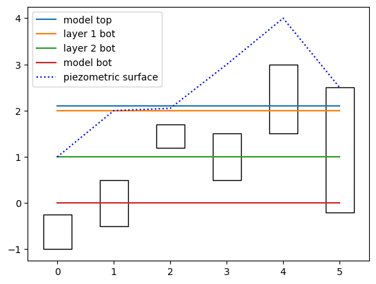
Plot the model top and layer bottoms (colors)

open intervals are shown as boxes * well 0 has zero transmissivities for each layer, as it is below the model bottom * well 1 has T values of 0 for layers 1 and 2, and 1 for layer 3 (K=2 x 0.5 thickness)

fig, ax = plt.subplots()
plt.plot(m.dis.top.array[r, c], label="model top")
for i, l in enumerate(m.dis.botm.array[:, r, c]):
    label = f"layer {i + 1} bot"
    if i == m.nlay - 1:
        label = "model bot"
    plt.plot(l, label=label)
plt.plot(heads[0], label="piezometric surface", color="b", linestyle=":")
for iw in range(len(sctop)):
    ax.fill_between(
        [iw - 0.25, iw + 0.25],
        scbot[iw],
        sctop[iw],
        facecolor="None",
        edgecolor="k",
    )
ax.legend(loc=2)

<matplotlib.legend.Legend at 0x7f1e8e0fff50>

example of transmissivites without sctop and scbot

• well zero has T=0 in layer 1 because it is dry; T=0.2 in layer 2 because the sat. thickness there is only 0.1

T = flopy.utils.get_transmissivities(heads, m, r=r, c=c)
np.round(T, 2)

array([[0. , 0. , 0.1, 0.2, 0.2, 0.2],
       [0.2, 2. , 2. , 2. , 2. , 2. ],
       [2. , 2. , 2. , 1.2, 2. , 2. ]])

try:
    # ignore PermissionError on Windows
    temp_dir.cleanup()
except:
    pass