Examples Gallery

The following examples illustrate the functionality of Flopy. After the tutorials, the examples are the best resource for learning the underlying capabilities of FloPy.

Preprocessing and Discretization

• Triangular mesh example
  • Creating Meshes with the Triangle Class
  • Specifying Regions with Different Triangle Sizes
  • Identifying Boundary Cells
  • Cell Attributes
  • Building a Simple MODFLOW 6 Model
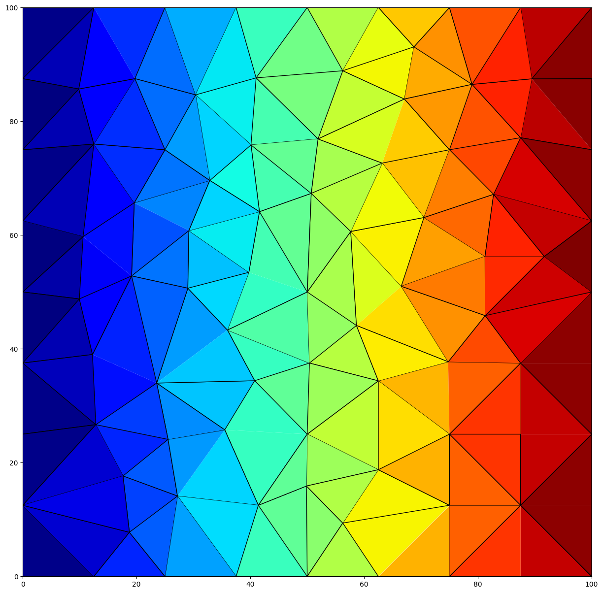
• Voronoi Grid and MODFLOW 6 Flow and Transport Example
  • Use Triangle to Generate Points for Voronoi Grid
  • Create and Plot FloPy Voronoi Grid
  • Use the VertexGrid Representation to Identify Boundary Cells
  • Create Run and Post Process a MODFLOW 6 Flow Model
  • Create Run and Post Process a MODFLOW 6 Transport Model
    • Building Voronoi Grid Examples
  • Irregular Domain Boundary
  • Simple Rectangular Domain
  • Circular Grid
  • Circular Grid with Hole
  • Regions with Different Refinement
  • Regions with Different Refinement and Hole
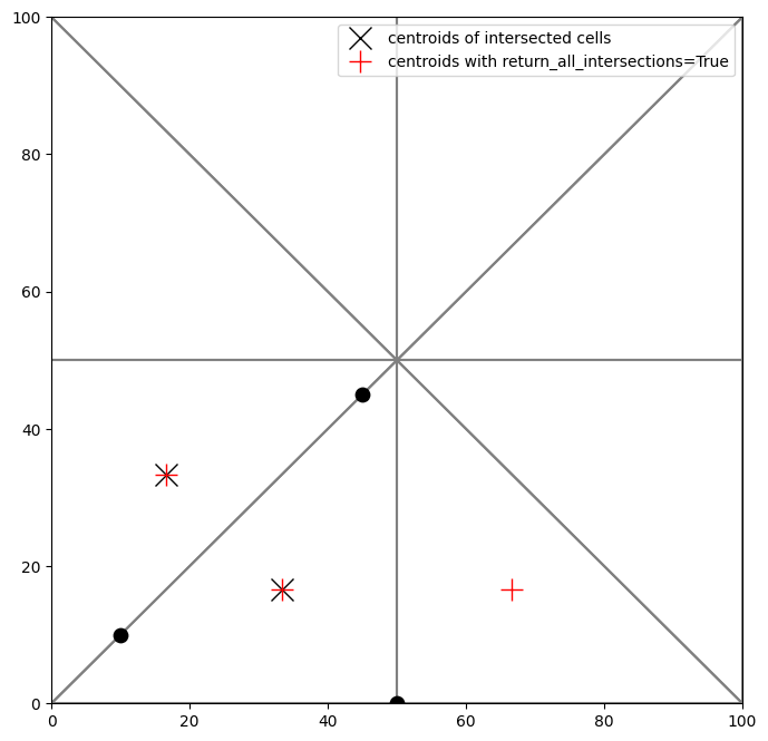
• Intersecting model grids with shapes
  • Table of Contents
    • GridIntersect Class
    • Rectangular regular grid
  • Polygon with regular grid
  • Polyline with regular grid
  • MultiPoint with regular grid
    • Vertex Grid
  • Polygon with triangular grid
  • LineString with triangular grid
  • MultiPoint with triangular grid
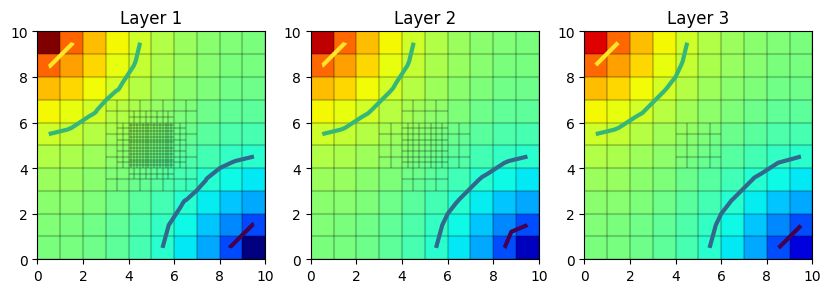
• Creating Layered Quadtree Grids with GRIDGEN
  • Import Modules and Locate Gridgen Executable
  • Basic Gridgen Operations
    • Setup Base MODFLOW Grid
    • Create the Gridgen Object
    • Add an Optional Active Domain
    • Refine the Grid
    • Plot the Gridgen Input
    • Build the Grid
    • Plot the Grid
    • Create a Flopy ModflowDisu Object
    • Intersect Features with the Grid
    • Plot Intersected Features
  • Use Gridgen to Build MODFLOW 6 DISV Model
  • Use Gridgen to Build MODFLOW 6 DISU Model
  • Use Gridgen to Build MODFLOW-USG DISU Model
• ModelGrid classes demo
  • The three modelgrid classes StructuredGrid, VertexGrid, and UnstructuredGrid will be demonstrated in this notebook.
    • This notebook will cover:
  • Accessing the modelgrid and common usage
    • How to access the modelgrid object from a model
      • Modflow-2005 example
      • Modflow-6 example
    • Accessing and setting modelgrid reference information
      • Accessing modelgrid reference information
      • Setting modelgrid reference information
    • Using the modelgrid with plotting routines
  • Building modelgrid objects from scratch
    • StructuredGrid example
      • In this example, some of the more common parameters are used to create a ``StructuredGrid``
      • Plot some of the modelgrid information
      • Plot a CrossSection of the structured grid
    • VertexGrid example
      • Building the VertexGrid
      • In this example, some of the more common parameters are used to create a ``VertexGrid``
      • Plot some of the modelgrid information
      • Plot a CrossSection of the vertex grid
    • UnstructuredGrid example
      • Building the UnstructuredGrid
      • In this example, some of the more common parameters are used to create a ``UnstructuredGrid``
      • Plot some of the modelgrid information
      • Plot a CrossSection of the unstructured grid
  • Useful methods and properties of the modelgrid classes
    • Common properties
      • Grid info properties
      • Spatial reference properties
      • Model discretization properties
    • Common methods
      • Overview of methods
      • set_coord_info()
      • get_coords()
      • get_local_coords()
      • intersect()
      • saturated_thickness()
      • write_shapefile()
• Intersecting rasters with modelgrids using FloPy’s Raster class
  • Raster files can be loaded using the Raster.load method
    • Intersecting and resampling a data using the FloPy ModelGrid
  • Structured Grid Example
    • Vertex and Unstructured grid example
    • Sampling points, Cropping, and performing intersections using raster data
  • Sampling points or a cross section from the raster
    • Sampling all points within a polygon in the raster
    • Cropping and resampling to a modelgrid
    • Arbitrary-shaped model boundaries
    • Future development

Triangular mesh example

Voronoi Grid and MODFLOW 6 Flow and Transport Example

Intersecting model grids with shapes

Creating Layered Quadtree Grids with GRIDGEN

ModelGrid classes demo

Intersecting rasters with modelgrids using FloPy’s Raster class

Postprocessing and Visualization

• Plotting SWR Process Results
  • Load SWR Process observations
    • Plot the data from the binary SWR Process observation file
  • Load the same data from the individual binary SWR Process files
    • Plot the data loaded from the individual binary SWR Process files.
  • Plot simulated water surface profiles
• Plotting Model Arrays and Results
  • Load and Run an Existing Model
  • Plotting Model Data
  • Plotting three-dimensional data
    • Plotting data for a single layer
  • Plotting transient two-dimensional data
    • Plotting data for a single stress period
  • Plotting simulated model results
    • Plotting results for a single layer
  • Passing other matplotlib.pyplot keywords to .plot() methods
  • Plotting data for a package or a model
  • Plot all data for a package
  • Plot package input data for a specified layer
  • Plot all input data for a model
  • Plot model input data for a specified layer
• Making Cross Sections of Your Model
  • Mapping is demonstrated for MODFLOW-2005 and MODFLOW-6 models in this notebook
  • Load and Run an Existing MODFLOW-2005 Model
  • Creating a Cross-Section of the Model Grid
  • Ploting Ibound
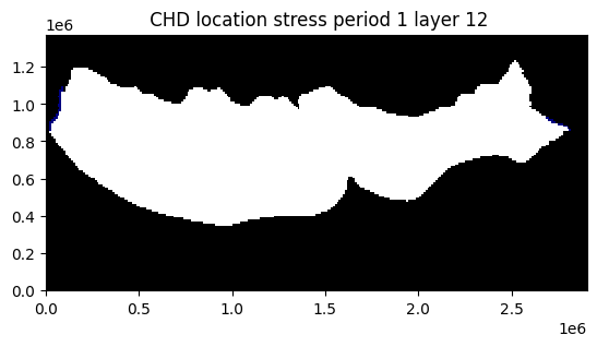
  • Plotting Boundary Conditions
  • Plotting an Array
  • Contouring an Array
  • Plotting Heads
  • Plotting a surface on the cross section
  • Plotting discharge vectors
  • Plotting a cross section from Shapefile data
  • Plotting geographic coordinates on the x-axis using the PlotCrossSection class
    • Plotting Cross Sections with MODFLOW-6 models
  • Plotting boundary conditions and arrays
  • Plotting specific discharge with a MODFLOW-6 model
    • Vertex cross section plotting with MODFLOW-6 (DISV)
  • Plotting a line based cross section through the model grid
  • Plotting Arrays and Contouring with Vertex Model grids
  • Plotting specific discharge vectors for DISV
    • Plotting using built in styles
    • Summary
• Making Maps of Your Model
  • Mapping is demonstrated for MODFLOW-2005, MODFLOW-USG, and MODFLOW-6 models in this notebook
  • Load and Run an Existing MODFLOW-2005 Model
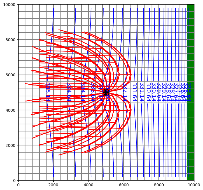
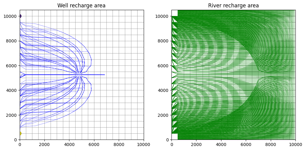
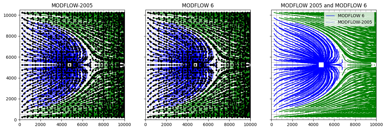
  • Create and Run MODPATH 6 model
  • Creating a Map of the Model Grid
    • Grid transformations and setting coordinate information
  • Ploting Ibound
  • Plotting Boundary Conditions
  • Plotting an Array
  • Contouring an Array
  • Plotting Heads
  • Plotting Discharge Vectors
  • Plotting MODPATH endpoints and pathlines
  • Plotting a Shapefile
  • Plotting GIS Shapes
    • Working with MODFLOW-6 models
  • Plotting boundary conditions and arrays
  • Contouring Arrays
  • Plotting specific discharge with a MODFLOW-6 model
    • Vertex model plotting with MODFLOW-6
  • Setting MODFLOW-6 Vertex Model Grid offsets, rotation and plotting
  • Plotting boundary conditions with Vertex Model grids
  • Plotting Arrays and Contouring with Vertex Model grids
  • Plotting MODPATH 7 results on a vertex model
  • Plotting specific discharge vectors for DISV
    • Unstructured grid (DISU) plotting with MODFLOW-USG and MODFLOW-6
    • Plotting using built in styles
    • Summary

Plotting SWR Process Results

Plotting Model Arrays and Results

Making Cross Sections of Your Model

Making Maps of Your Model

Exporting data

• Shapefile export demo
  • set the model coordinate information
    • Declarative export using attached .export() methods
      • Export the whole model to a single shapefile
  • Export a package to a shapefile
  • Export a FloPy list or array object
  • MfList.export() exports the whole grid by default, regardless of the locations of the boundary cells
    • Ad-hoc exporting using recarray2shp
  • combining data from different packages
  • exporting other data
  • Adding attribute data to an existing shapefile
    • Overriding the model’s modelgrid with a user supplied modelgrid

Shapefile export demo

Other FloPy features

• FloPy working stack demo
  • Model Inputs
  • Inspecting outputs
• Computing transmissivity-weighted averages
  • Make up some open interval tops and bottoms and some heads
  • Make a flopy modflow model
  • Get transmissivities along the diagonal cells
  • Plot the model top and layer bottoms (colors)
  • example of transmissivites without sctop and scbot
• Saving array data to MODFLOW-style binary files
• Working with shapefiles
  • write a numpy record array to a shapefile
  • set coordinate information
  • make geometry objects for the cells with errors
  • write the shapefile
  • read it back in
    • Other geometry types
  • Linestring
    • Points

FloPy working stack demo

Computing transmissivity-weighted averages

Saving array data to MODFLOW-style binary files

Working with shapefiles

MODFLOW 6 examples

• Creating a Complex MODFLOW 6 Model with Flopy
  • Setup the Notebook Environment
  • Create the MODFLOW 6 Input Files and Run the Model
  • Run the Simulation
  • Post-Process Head Results
  • Post-Process Flows
  • Post-Process Head Observations
• Model splitting for parallel and serial MODFLOW 6
  • Example 1: splitting a simple structured grid model
    • Creating an array that defines the new models
    • Splitting the model using Mf6Splitter()
    • Visualize and reassemble model output
    • Array based model output can be assembled into the original model’s shape by using the reconstruct_array() method
    • Recarray based model inputs and outputs can also be assembled into the original model’s shape by using the reconstruct_recarray() method
  • Example 2: a more comprehensive example with the watershed model from Hughes and others 2023
    • Create the model
    • Split the watershed model
    • Now split the model into many models using Mf6Splitter()
    • Reassemble the heads to the original model shape for plotting
  • Example 3: create an optimized splitting mask for a model
    • Reassemble the heads and plot results
• Creating a Simple MODFLOW 6 Model with Flopy
  • Setup the Notebook Environment
  • Create the Flopy Model Objects
  • Create the MODFLOW 6 Input Files and Run the Model
  • Run the Simulation
  • Post-Process Head Results
  • Post-Process Flows
• Flopy MODFLOW 6 (MF6) Support
  • Conceptual model
    • flopy.mf6.MFSimulation
    • flopy.mf6.ModflowGwf
    • flopy.mf6.Modflow[pc]
  • Creating a simulation
  • Accessing namefiles
  • Specifying options
  • MFArray templates
  • Specifying MFArray Data
  • MFList Templates
  • Cell IDs
  • Specifying MFList Data
    • Specifying MFList Data in an External File
  • Packages that Support both List-based and Array-based Data
  • Utility Files (TS, TAS, OBS, TAB)
  • Saving and Running a MF6 Simulation
  • Exporting a MF6 Model
  • Loading an Existing MF6 Simulation
  • Retrieving Data and Modifying an Existing MF6 Simulation
  • Modifying Data
  • Modifying the Simulation Path
  • Adding a Model Relative Path
  • Post-Processing the Results

Creating a Complex MODFLOW 6 Model with Flopy

Model splitting for parallel and serial MODFLOW 6

Creating a Simple MODFLOW 6 Model with Flopy

Flopy MODFLOW 6 (MF6) Support

MODFLOW USG examples

• MODFLOW-USG CLN package demo
  • Loading Example 03_conduit_confined
  • Create example 03A_conduit_unconfined of mfusg 1.5
  • Modify CLN amd WEL package to example create 03B_conduit_unconfined of mfusg 1.5
  • Modify CLN amd WEL package to example create 03C_conduit_unconfined of mfusg 1.5
  • Modify CLN amd WEL package to example create 03D_conduit_unconfined of mfusg 1.5
  • Comparing four cases
• MODFLOW-USG Freyberg demo
• MODFLOW-USG: Discontinuous water table configuration over a stairway impervious base
  • Model parameters
  • Create and run the MODFLOW-USG model
    • Read the simulated MODFLOW-USG model results
    • Plot MODFLOW-USG results

MODFLOW-USG CLN package demo

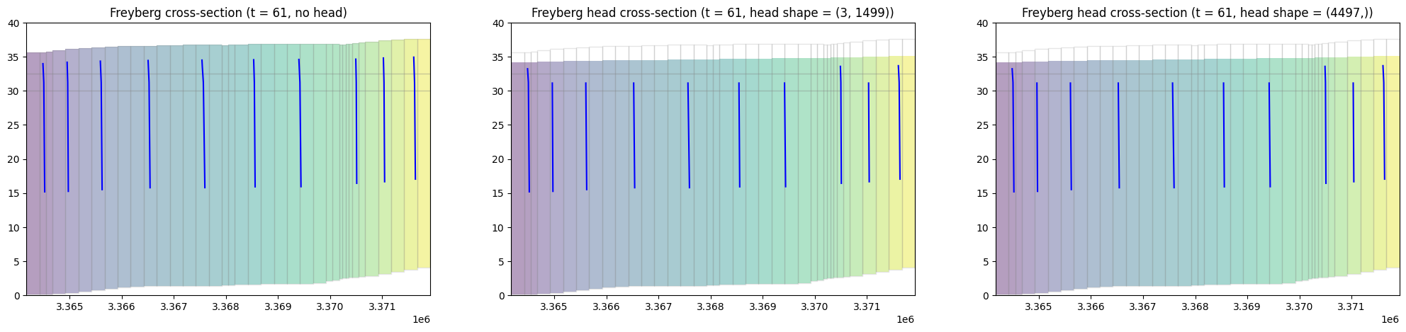
MODFLOW-USG Freyberg demo

MODFLOW-USG: Discontinuous water table configuration over a stairway impervious base

MODFLOW-2005/MODFLOW-NWT examples

• Flopy Drain Return (DRT) capabilities
• Lake Package Example
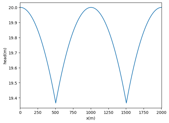
• Simple water-table solution with recharge
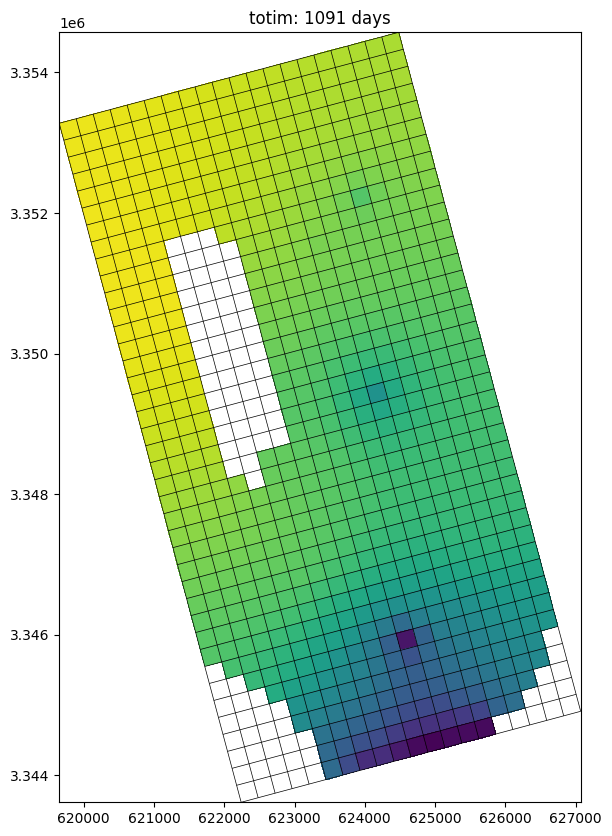
• Postprocessing head results from MODFLOW
  • Load example model and head results
  • Plot heads in each layer; export the heads and head contours for viewing in a GIS
  • Compare rotated arc-ascii and GeoTiff output
  • Get the vertical head gradients between layers
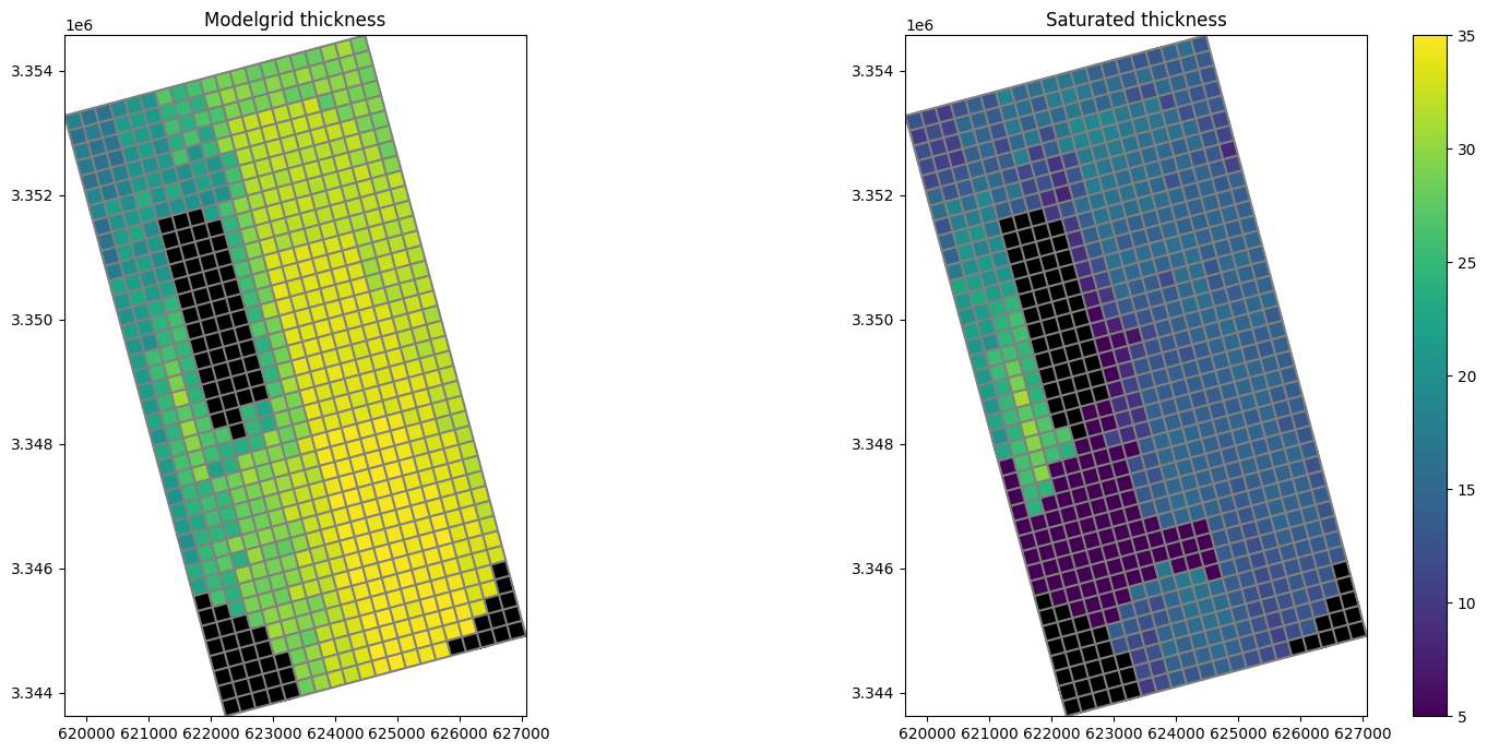
  • Get the saturated thickness of a layer
  • Get the water table
  • Get layer transmissivities at arbitrary locations, accounting for the position of the water table
    • convert to transmissivity fractions
    • Layer 3 contributes almost no transmissivity because of its K-value
• SFR package Prudic and others (2004) example
  • Problem description:
  • copy over the example files to the working directory
    • Load example dataset, skipping the SFR package
    • Read pre-prepared reach and segment data into numpy recarrays using numpy.genfromtxt()
    • Segment Data structure
    • define dataset 6e (channel flow data) for segment 1
    • define dataset 6d (channel geometry data) for segments 7 and 8
    • Define SFR package variables
    • Instantiate SFR package
    • Plot the SFR segments
    • Check the SFR dataset for errors
    • Load SFR formated water balance output into pandas dataframe using the SfrFile class
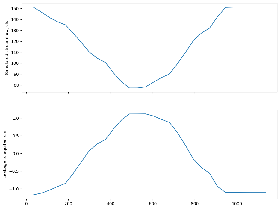
  • Plot streamflow and stream/aquifer interactions for a segment
    • Look at stage, model top, and streambed top
    • Get SFR leakage results from cell budget file
    • Plot leakage in plan view
    • Plot total streamflow
      • Reading transient SFR formatted output
    • plot a hydrograph
• SWI2 Example 1. Rotating Interface
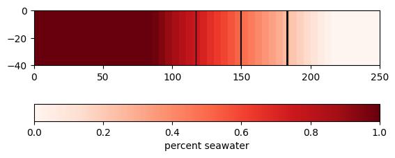
• SWI2 Example 4. Upconing Below a Pumping Well in a Two-Aquifer Island System
• Unsaturated Zone Flow (UZF) Package demo
  • Problem description:
    • Set up the gages (observation points)
      • Inspecting results

Flopy Drain Return (DRT) capabilities

Lake Package Example

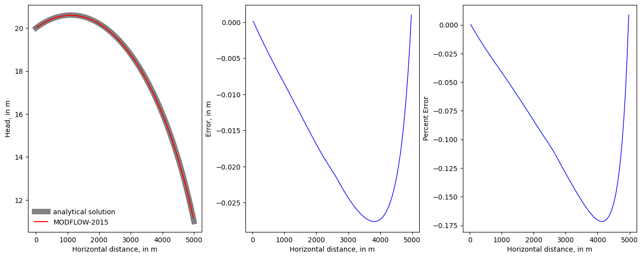
Simple water-table solution with recharge

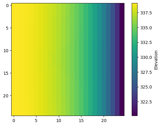
Postprocessing head results from MODFLOW

SFR package Prudic and others (2004) example

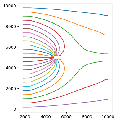
SWI2 Example 1. Rotating Interface

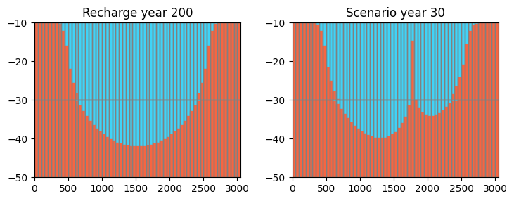
SWI2 Example 4. Upconing Below a Pumping Well in a Two-Aquifer Island System

Unsaturated Zone Flow (UZF) Package demo

MODPATH examples

• Working with MODPATH 6
• Creating a MODPATH 7 simulation
  • Flow model data
  • MODPATH 7 using MODFLOW 6
    • Create and run MODFLOW 6
    • Create and run MODPATH 7
    • Load and Plot MODPATH 7 output
      • Forward Tracking
      • Backward tracking
• Using MODPATH 7 with structured grids
  • Flow model data
  • MODPATH 7 data
  • MODPATH 7 using MODFLOW-2005
    • Create and run MODFLOW-2005
    • Create and run MODPATH 7
    • Load MODPATH 7 output
    • Plot MODPATH 7 output
  • MODPATH 7 using MODFLOW 6
    • Create and run MODFLOW 6
    • Create and run MODPATH 7
    • Load MODPATH 7 output
  • Plot MODPATH 7 output
  • Compare MODPATH results
• Using MODPATH 7 with structured grids (transient example)
  • Setting up the simulation
  • Running the simulation
  • Inspecting results
• Using MODPATH 7 with a DISV unstructured model
  • Part I. Setup Notebook
  • Part II. Gridgen Creation of Model Grid
  • Part III. Create the Flopy Model
  • Part IV. Run the MODFLOW 6 Model
  • Part V. Import and Plot the Results
  • Part VI. Create the Flopy MODPATH7 Models
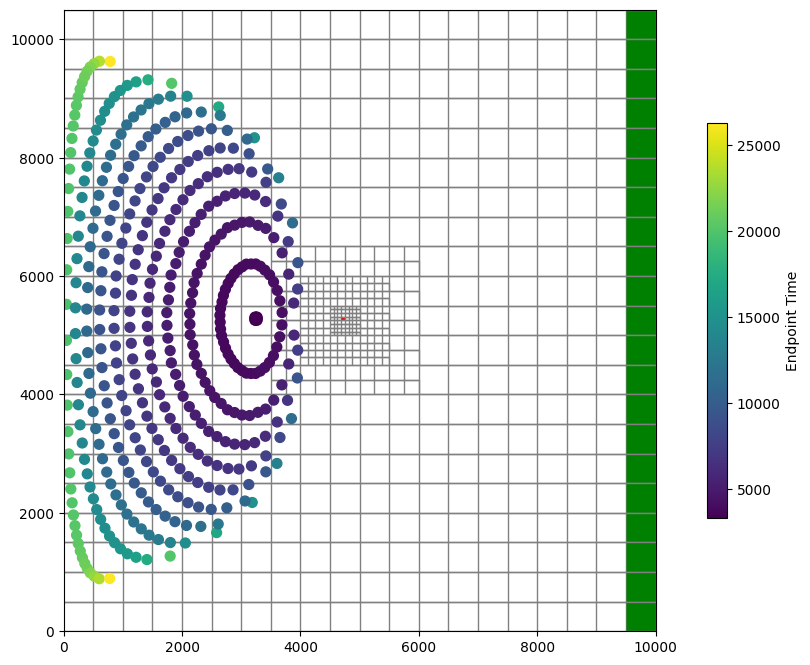
• Using MODPATH 7: DISV quadpatch example
  • Grid creation/refinement
  • Groundwater flow model
  • Particle tracking
• FloPy VTK/PyVista particle tracking pathline visualization demo

Working with MODPATH 6

Creating a MODPATH 7 simulation

Using MODPATH 7 with structured grids

Using MODPATH 7 with structured grids (transient example)

Using MODPATH 7 with a DISV unstructured model

Using MODPATH 7: DISV quadpatch example

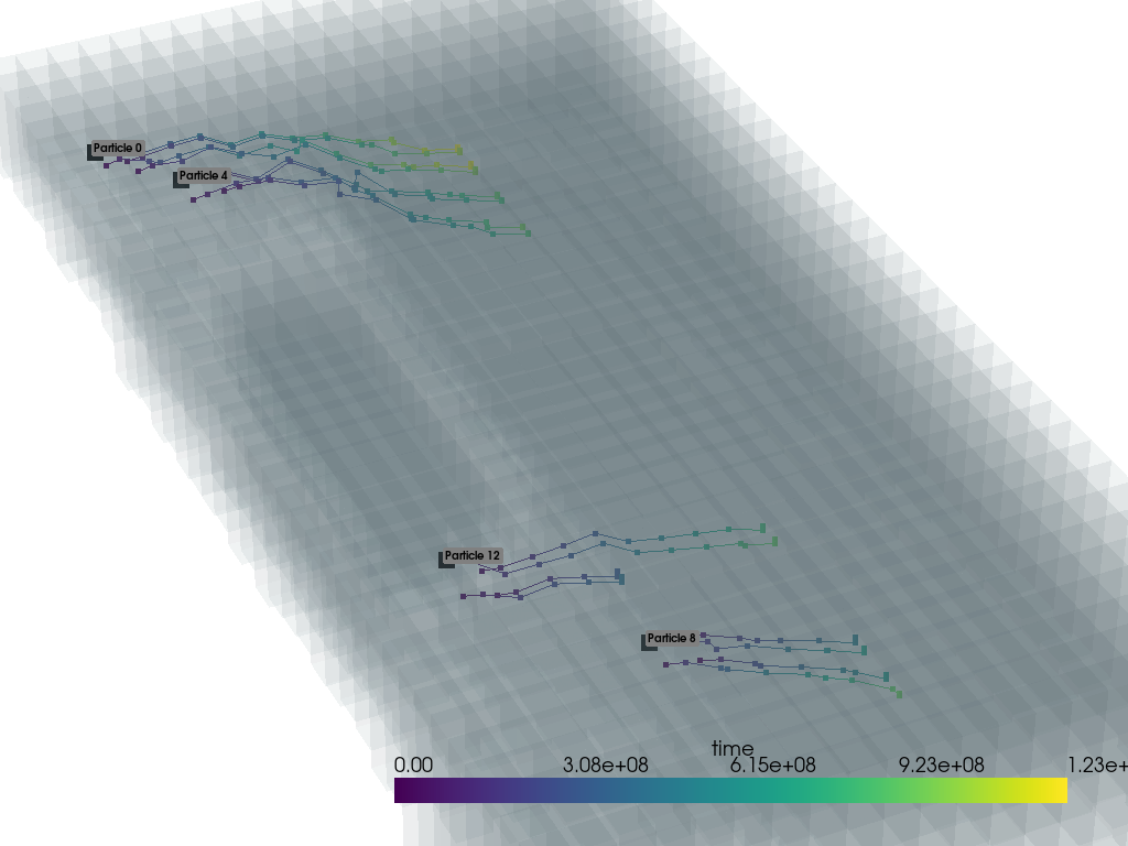
FloPy VTK/PyVista particle tracking pathline visualization demo

MT3D and SEAWAT examples

• MT3D-USGS Example
  • Problem description:
    • Compare mt3d-usgs results to an analytical solution
• MT3DMS Example Problems
  • Example 1. One-Dimensional Transport in a Uniform Flow Field
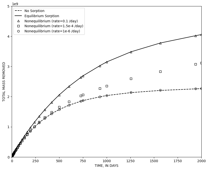
  • Example 2. One-Dimensional Transport with Nonlinear or Nonequilibrium Sorption
  • Example 3. Two-Dimensional Transport in a Uniform Flow Field
  • Example 4. Two-Dimensional Transport in a Diagonal Flow Field
  • Example 5. Two-Dimensional Transport in a Radial Flow Field
  • Example 6. Concentration at an Injection/Extraction Well
  • Example 7. Three-Dimensional Transport in a Uniform Flow Field
  • Example 8. Two-Dimensional, Vertical Transport in a Heterogeneous Aquifer
  • Example 9. Two-Dimensional Application Example
  • Example 10. Three-Dimensional Field Case Study

MT3D-USGS Example

MT3DMS Example Problems

Examples from Bakker and others (2016)

• Basic Flopy example
• Capture fraction example

Basic Flopy example

Capture fraction example

Examples from Hughes and others (2023)

• Watershed geoprocessing example
  • Structured Grids
    • Structured grid with constant row and column spacing
    • Structured grid with variable row and column spacing
    • Local grid refinement grid
  • Unstructured grids
    • Quadtree grid
    • Triangular grid
    • Voronoi Grid from the Triangle object
  • Plot all six grids
    • Create a polyline for Local Grid Refinement area
    • Plot the grids
    • Plot the river intersection for the six grids

Watershed geoprocessing example

Miscellaneous examples

• Henry Saltwater Intrusion Problem
  • Change the format of several arrays and rerun the model
• ZoneBudget Example
  • Read File Containing Zones
  • Extract Budget Information from ZoneBudget Object
  • Convert Units
  • Alias Names
  • Return the Budgets as a Pandas DataFrame
  • Write Budget Output to CSV
  • Net Budget
  • Plot Budget Components
    • Zonebudget for Modflow 6 (ZoneBudget6)
  • Use the the .output model attribute to create a zonebudget model
  • Getting the zonebudget output

Henry Saltwater Intrusion Problem

ZoneBudget Example