Using MODPATH 7 with a DISV unstructured model
This is a replication of the MODPATH Problem 2 example that is described on page 12 of the modpath_7_examples.pdf file. The results shown here should be the same as the results in the MODPATH example, however, the vertex and node numbering used here may be different from the numbering used in MODPATH, so head values may not be compared directly without some additional mapping.
Part I. Setup Notebook
[1]:
import os
[2]:
import sys
from pathlib import Path
from tempfile import TemporaryDirectory

import matplotlib as mpl
import matplotlib.pyplot as plt
import numpy as np

proj_root = Path.cwd().parent.parent

import flopy

print(sys.version)
print(f"numpy version: {np.__version__}")
print(f"matplotlib version: {mpl.__version__}")
print(f"flopy version: {flopy.__version__}")

# temporary directory
temp_dir = TemporaryDirectory()
workspace = Path(temp_dir.name)
3.12.2 | packaged by conda-forge | (main, Feb 16 2024, 20:50:58) [GCC 12.3.0]
numpy version: 1.26.4
matplotlib version: 3.8.4
flopy version: 3.7.0.dev0
Part II. Gridgen Creation of Model Grid
Create the base model grid.
[3]:
Lx = 10000.0
Ly = 10500.0
nlay = 3
nrow = 21
ncol = 20
delr = Lx / ncol
delc = Ly / nrow
top = 400
botm = [220, 200, 0]
[4]:
ms = flopy.modflow.Modflow()
dis5 = flopy.modflow.ModflowDis(
    ms,
    nlay=nlay,
    nrow=nrow,
    ncol=ncol,
    delr=delr,
    delc=delc,
    top=top,
    botm=botm,
)
Create the Gridgen object.
[5]:
from flopy.utils.gridgen import Gridgen

model_name = "mp7p2_u"
model_ws = workspace / "mp7_ex2" / "mf6"
gridgen_ws = model_ws / "gridgen"
g = Gridgen(ms.modelgrid, model_ws=gridgen_ws)
Refine the grid.
[6]:
rf0shp = gridgen_ws / "rf0"
xmin = 7 * delr
xmax = 12 * delr
ymin = 8 * delc
ymax = 13 * delc
rfpoly = [
    [
        list(
            reversed(
                [
                    (xmin, ymin),
                    (xmax, ymin),
                    (xmax, ymax),
                    (xmin, ymax),
                    (xmin, ymin),
                ]
            )
        )
    ]
]
g.add_refinement_features(rfpoly, "polygon", 1, range(nlay))

rf1shp = gridgen_ws / "rf1"
xmin = 8 * delr
xmax = 11 * delr
ymin = 9 * delc
ymax = 12 * delc
rfpoly = [
    [
        list(
            reversed(
                [
                    (xmin, ymin),
                    (xmax, ymin),
                    (xmax, ymax),
                    (xmin, ymax),
                    (xmin, ymin),
                ]
            )
        )
    ]
]
g.add_refinement_features(rfpoly, "polygon", 2, range(nlay))

rf2shp = gridgen_ws / "rf2"
xmin = 9 * delr
xmax = 10 * delr
ymin = 10 * delc
ymax = 11 * delc
rfpoly = [
    [
        list(
            reversed(
                [
                    (xmin, ymin),
                    (xmax, ymin),
                    (xmax, ymax),
                    (xmin, ymax),
                    (xmin, ymin),
                ]
            )
        )
    ]
]
g.add_refinement_features(rfpoly, "polygon", 3, range(nlay))
Show the model grid with refinement levels superimposed.
[7]:
fig = plt.figure(figsize=(5, 5), constrained_layout=True)
ax = fig.add_subplot(1, 1, 1)
mm = flopy.plot.PlotMapView(model=ms)
mm.plot_grid()
flopy.plot.plot_shapefile(rf0shp, ax=ax, facecolor="yellow", edgecolor="none")
flopy.plot.plot_shapefile(rf1shp, ax=ax, facecolor="pink", edgecolor="none")
flopy.plot.plot_shapefile(rf2shp, ax=ax, facecolor="red", edgecolor="none")
[7]:
<matplotlib.collections.PatchCollection at 0x7fe49f1a4770>

Build the refined grid.
[8]:
g.build(verbose=False)
Show the refined grid.
[9]:
fig = plt.figure(figsize=(5, 5), constrained_layout=True)
ax = fig.add_subplot(1, 1, 1, aspect="equal")
g.plot(ax, linewidth=0.5)
[9]:
<matplotlib.collections.PatchCollection at 0x7fe4a176b560>

Extract the refined grid’s properties.
[10]:
gridprops = g.get_gridprops_disv()
ncpl = gridprops["ncpl"]
top = gridprops["top"]
botm = gridprops["botm"]
nvert = gridprops["nvert"]
vertices = gridprops["vertices"]
cell2d = gridprops["cell2d"]
Part III. Create the Flopy Model
[11]:
# create simulation
sim = flopy.mf6.MFSimulation(
    sim_name=model_name, version="mf6", exe_name="mf6", sim_ws=model_ws
)

# create tdis package
tdis_rc = [(1000.0, 1, 1.0)]
tdis = flopy.mf6.ModflowTdis(
    sim, pname="tdis", time_units="DAYS", perioddata=tdis_rc
)

# create gwf model
gwf = flopy.mf6.ModflowGwf(
    sim, modelname=model_name, model_nam_file=f"{model_name}.nam"
)
gwf.name_file.save_flows = True

# create iterative model solution and register the gwf model with it
ims = flopy.mf6.ModflowIms(
    sim,
    pname="ims",
    print_option="SUMMARY",
    complexity="SIMPLE",
    outer_dvclose=1.0e-5,
    outer_maximum=100,
    under_relaxation="NONE",
    inner_maximum=100,
    inner_dvclose=1.0e-6,
    rcloserecord=0.1,
    linear_acceleration="BICGSTAB",
    scaling_method="NONE",
    reordering_method="NONE",
    relaxation_factor=0.99,
)
sim.register_ims_package(ims, [gwf.name])

# disv
disv = flopy.mf6.ModflowGwfdisv(
    gwf,
    nlay=nlay,
    ncpl=ncpl,
    top=top,
    botm=botm,
    nvert=nvert,
    vertices=vertices,
    cell2d=cell2d,
)

# initial conditions
ic = flopy.mf6.ModflowGwfic(gwf, pname="ic", strt=320.0)

# node property flow
npf = flopy.mf6.ModflowGwfnpf(
    gwf,
    xt3doptions=[("xt3d")],
    icelltype=[1, 0, 0],
    k=[50.0, 0.01, 200.0],
    k33=[10.0, 0.01, 20.0],
)

# wel
wellpoints = [(4750.0, 5250.0)]
welcells = g.intersect(wellpoints, "point", 0)
# welspd = flopy.mf6.ModflowGwfwel.stress_period_data.empty(gwf, maxbound=1, aux_vars=['iface'])
welspd = [[(2, icpl), -150000, 0] for icpl in welcells["nodenumber"]]
wel = flopy.mf6.ModflowGwfwel(
    gwf, print_input=True, auxiliary=[("iface",)], stress_period_data=welspd
)

# rch
aux = [np.ones(ncpl, dtype=int) * 6]
rch = flopy.mf6.ModflowGwfrcha(
    gwf, recharge=0.005, auxiliary=[("iface",)], aux={0: [6]}
)
# riv
riverline = [[(Lx - 1.0, Ly), (Lx - 1.0, 0.0)]]
rivcells = g.intersect(riverline, "line", 0)
rivspd = [[(0, icpl), 320.0, 100000.0, 318] for icpl in rivcells["nodenumber"]]
riv = flopy.mf6.ModflowGwfriv(gwf, stress_period_data=rivspd)

# output control
oc = flopy.mf6.ModflowGwfoc(
    gwf,
    pname="oc",
    budget_filerecord=f"{model_name}.cbb",
    head_filerecord=f"{model_name}.hds",
    headprintrecord=[("COLUMNS", 10, "WIDTH", 15, "DIGITS", 6, "GENERAL")],
    saverecord=[("HEAD", "ALL"), ("BUDGET", "ALL")],
    printrecord=[("HEAD", "ALL"), ("BUDGET", "ALL")],
)
Now write the simulation input files.
[12]:
sim.write_simulation()
writing simulation...
  writing simulation name file...
  writing simulation tdis package...
  writing solution package ims...
  writing model mp7p2_u...
    writing model name file...
    writing package disv...
    writing package ic...
    writing package npf...
    writing package wel_0...
INFORMATION: maxbound in ('gwf6', 'wel', 'dimensions') changed to 1 based on size of stress_period_data
    writing package rcha_0...
    writing package riv_0...
INFORMATION: maxbound in ('gwf6', 'riv', 'dimensions') changed to 21 based on size of stress_period_data
    writing package oc...
Part IV. Run the MODFLOW 6 Model
[13]:
success, buff = sim.run_simulation(silent=True, report=True)
assert success, "mf6 failed to run"
for line in buff:
    print(line)
                                   MODFLOW 6
                U.S. GEOLOGICAL SURVEY MODULAR HYDROLOGIC MODEL
                            VERSION 6.4.4 02/13/2024

   MODFLOW 6 compiled Feb 19 2024 14:19:54 with Intel(R) Fortran Intel(R) 64
   Compiler Classic for applications running on Intel(R) 64, Version 2021.7.0
                             Build 20220726_000000

This software has been approved for release by the U.S. Geological
Survey (USGS). Although the software has been subjected to rigorous
review, the USGS reserves the right to update the software as needed
pursuant to further analysis and review. No warranty, expressed or
implied, is made by the USGS or the U.S. Government as to the
functionality of the software and related material nor shall the
fact of release constitute any such warranty. Furthermore, the
software is released on condition that neither the USGS nor the U.S.
Government shall be held liable for any damages resulting from its
authorized or unauthorized use. Also refer to the USGS Water
Resources Software User Rights Notice for complete use, copyright,
and distribution information.


 Run start date and time (yyyy/mm/dd hh:mm:ss): 2024/05/17  1:01:27

 Writing simulation list file: mfsim.lst
 Using Simulation name file: mfsim.nam

    Solving:  Stress period:     1    Time step:     1

 Run end date and time (yyyy/mm/dd hh:mm:ss): 2024/05/17  1:01:28
 Elapsed run time:  0.097 Seconds

 Normal termination of simulation.
Part V. Import and Plot the Results
Plot the boundary conditions on the grid.
[14]:
fname = os.path.join(model_ws, f"{model_name}.disv.grb")
grd = flopy.mf6.utils.MfGrdFile(fname, verbose=False)
mg = grd.modelgrid
ibd = np.zeros((ncpl), dtype=int)
ibd[welcells["nodenumber"]] = 1
ibd[rivcells["nodenumber"]] = 2
ibd = np.ma.masked_equal(ibd, 0)
fig = plt.figure(figsize=(8, 8), constrained_layout=True)
ax = fig.add_subplot(1, 1, 1, aspect="equal")
pmv = flopy.plot.PlotMapView(modelgrid=mg, ax=ax)
ax.set_xlim(0, Lx)
ax.set_ylim(0, Ly)
cmap = mpl.colors.ListedColormap(
    [
        "r",
        "g",
    ]
)
pc = pmv.plot_array(ibd, cmap=cmap, edgecolor="gray")
t = ax.set_title("Boundary Conditions\n")

[15]:
fname = os.path.join(model_ws, f"{model_name}.hds")
hdobj = flopy.utils.HeadFile(fname)
head = hdobj.get_data()
head.shape
[15]:
(3, 1, 651)
[16]:
ilay = 2
cint = 0.25
fig = plt.figure(figsize=(8, 8), constrained_layout=True)
ax = fig.add_subplot(1, 1, 1, aspect="equal")
mm = flopy.plot.PlotMapView(modelgrid=mg, ax=ax, layer=ilay)
ax.set_xlim(0, Lx)
ax.set_ylim(0, Ly)
pc = mm.plot_array(head[:, 0, :], cmap="jet", edgecolor="black")
hmin = head[ilay, 0, :].min()
hmax = head[ilay, 0, :].max()
levels = np.arange(np.floor(hmin), np.ceil(hmax) + cint, cint)
cs = mm.contour_array(head[:, 0, :], colors="white", levels=levels)
plt.clabel(cs, fmt="%.1f", colors="white", fontsize=11)
cb = plt.colorbar(pc, shrink=0.5)
t = ax.set_title(f"Model Layer {ilay + 1}; hmin={hmin:6.2f}, hmax={hmax:6.2f}")

Inspect model cells and vertices.
[17]:
# zoom area
xmin, xmax = 2000, 4500
ymin, ymax = 5400, 7500

mg.get_cell_vertices
fig = plt.figure(figsize=(8, 8), constrained_layout=True)
ax = fig.add_subplot(1, 1, 1, aspect="equal")
mm = flopy.plot.PlotMapView(modelgrid=mg, ax=ax)
v = mm.plot_grid(edgecolor="black")
t = ax.set_title("Model Cells and Vertices (one-based)\n")
ax.set_xlim(xmin, xmax)
ax.set_ylim(ymin, ymax)

verts = mg.verts
ax.plot(verts[:, 0], verts[:, 1], "bo")
for i in range(ncpl):
    x, y = verts[i, 0], verts[i, 1]
    if xmin <= x <= xmax and ymin <= y <= ymax:
        ax.annotate(str(i + 1), verts[i, :], color="b")

xc, yc = mg.get_xcellcenters_for_layer(0), mg.get_ycellcenters_for_layer(0)
for i in range(ncpl):
    x, y = xc[i], yc[i]
    ax.plot(x, y, "ro")
    if xmin <= x <= xmax and ymin <= y <= ymax:
        ax.annotate(str(i + 1), (x, y), color="r")

Part VI. Create the Flopy MODPATH7 Models
Define names for the MODPATH 7 simulations.
[18]:
mp_namea = f"{model_name}a_mp"
mp_nameb = f"{model_name}b_mp"
Create particles for the pathline and timeseries analysis.
[19]:
pcoord = np.array(
    [
        [0.000, 0.125, 0.500],
        [0.000, 0.375, 0.500],
        [0.000, 0.625, 0.500],
        [0.000, 0.875, 0.500],
        [1.000, 0.125, 0.500],
        [1.000, 0.375, 0.500],
        [1.000, 0.625, 0.500],
        [1.000, 0.875, 0.500],
        [0.125, 0.000, 0.500],
        [0.375, 0.000, 0.500],
        [0.625, 0.000, 0.500],
        [0.875, 0.000, 0.500],
        [0.125, 1.000, 0.500],
        [0.375, 1.000, 0.500],
        [0.625, 1.000, 0.500],
        [0.875, 1.000, 0.500],
    ]
)
nodew = gwf.disv.ncpl.array * 2 + welcells["nodenumber"][0]
plocs = [nodew for i in range(pcoord.shape[0])]

# create particle data
pa = flopy.modpath.ParticleData(
    plocs,
    structured=False,
    localx=pcoord[:, 0],
    localy=pcoord[:, 1],
    localz=pcoord[:, 2],
    drape=0,
)

# create backward particle group
fpth = f"{mp_namea}.sloc"
pga = flopy.modpath.ParticleGroup(
    particlegroupname="BACKWARD1", particledata=pa, filename=fpth
)
Create particles for endpoint analysis.
[20]:
facedata = flopy.modpath.FaceDataType(
    drape=0,
    verticaldivisions1=10,
    horizontaldivisions1=10,
    verticaldivisions2=10,
    horizontaldivisions2=10,
    verticaldivisions3=10,
    horizontaldivisions3=10,
    verticaldivisions4=10,
    horizontaldivisions4=10,
    rowdivisions5=0,
    columndivisions5=0,
    rowdivisions6=4,
    columndivisions6=4,
)
pb = flopy.modpath.NodeParticleData(subdivisiondata=facedata, nodes=nodew)
# create forward particle group
fpth = f"{mp_nameb}.sloc"
pgb = flopy.modpath.ParticleGroupNodeTemplate(
    particlegroupname="BACKWARD2", particledata=pb, filename=fpth
)
Create and run the pathline and timeseries analysis model.
[21]:
# create modpath files
mp = flopy.modpath.Modpath7(
    modelname=mp_namea, flowmodel=gwf, exe_name="mp7", model_ws=model_ws
)
flopy.modpath.Modpath7Bas(mp, porosity=0.1)
flopy.modpath.Modpath7Sim(
    mp,
    simulationtype="combined",
    trackingdirection="backward",
    weaksinkoption="pass_through",
    weaksourceoption="pass_through",
    referencetime=0.0,
    stoptimeoption="extend",
    timepointdata=[500, 1000.0],
    particlegroups=pga,
)

# write modpath datasets
mp.write_input()

# run modpath
success, buff = mp.run_model(silent=True, report=True)
assert success, "mp7 failed to run"
for line in buff:
    print(line)
MODPATH Version 7.2.001
Program compiled Feb 19 2024 14:21:54 with IFORT compiler (ver. 20.21.7)


Run particle tracking simulation ...
Processing Time Step     1 Period     1.  Time =  1.00000E+03  Steady-state flow

Particle Summary:
         0 particles are pending release.
         0 particles remain active.
        16 particles terminated at boundary faces.
         0 particles terminated at weak sink cells.
         0 particles terminated at weak source cells.
         0 particles terminated at strong source/sink cells.
         0 particles terminated in cells with a specified zone number.
         0 particles were stranded in inactive or dry cells.
         0 particles were unreleased.
         0 particles have an unknown status.

Normal termination.
Load the pathline and timeseries data.
[22]:
fpth = model_ws / f"{mp_namea}.mppth"
p = flopy.utils.PathlineFile(fpth)
p0 = p.get_alldata()
[23]:
fpth = model_ws / f"{mp_namea}.timeseries"
ts = flopy.utils.TimeseriesFile(fpth)
ts0 = ts.get_alldata()
Plot the pathline and timeseries data.
[24]:
fig = plt.figure(figsize=(8, 8), constrained_layout=True)
ax = fig.add_subplot(1, 1, 1, aspect="equal")
mm = flopy.plot.PlotMapView(modelgrid=mg, ax=ax)
ax.set_xlim(0, Lx)
ax.set_ylim(0, Ly)
cmap = mpl.colors.ListedColormap(
    [
        "r",
        "g",
    ]
)
v = mm.plot_array(ibd, cmap=cmap, edgecolor="gray")
mm.plot_pathline(p0, layer="all", colors="blue", lw=0.75)
colors = ["green", "orange", "red"]
for k in range(nlay):
    mm.plot_timeseries(ts0, layer=k, marker="o", lw=0, color=colors[k])

Create and run the endpoint analysis model.
[25]:
# create modpath files
mp = flopy.modpath.Modpath7(
    modelname=mp_nameb, flowmodel=gwf, exe_name="mp7", model_ws=model_ws
)
flopy.modpath.Modpath7Bas(mp, porosity=0.1)
flopy.modpath.Modpath7Sim(
    mp,
    simulationtype="endpoint",
    trackingdirection="backward",
    weaksinkoption="pass_through",
    weaksourceoption="pass_through",
    referencetime=0.0,
    stoptimeoption="extend",
    particlegroups=pgb,
)

# write modpath datasets
mp.write_input()

# run modpath
success, buff = mp.run_model(silent=True, report=True)
assert success, "mp7 failed to run"
for line in buff:
    print(line)
MODPATH Version 7.2.001
Program compiled Feb 19 2024 14:21:54 with IFORT compiler (ver. 20.21.7)


Run particle tracking simulation ...
Processing Time Step     1 Period     1.  Time =  1.00000E+03  Steady-state flow

Particle Summary:
         0 particles are pending release.
         0 particles remain active.
       416 particles terminated at boundary faces.
         0 particles terminated at weak sink cells.
         0 particles terminated at weak source cells.
         0 particles terminated at strong source/sink cells.
         0 particles terminated in cells with a specified zone number.
         0 particles were stranded in inactive or dry cells.
         0 particles were unreleased.
         0 particles have an unknown status.

Normal termination.
Load the endpoint data.
[26]:
fpth = model_ws / f"{mp_nameb}.mpend"
e = flopy.utils.EndpointFile(fpth)
e0 = e.get_alldata()
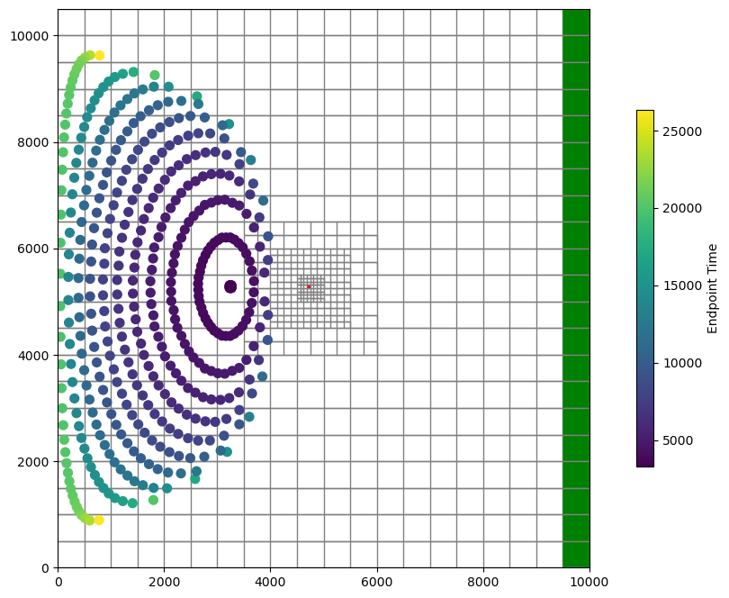
Plot the endpoint data.
[27]:
fig = plt.figure(figsize=(8, 8), constrained_layout=True)
ax = fig.add_subplot(1, 1, 1, aspect="equal")
mm = flopy.plot.PlotMapView(modelgrid=mg, ax=ax)
ax.set_xlim(0, Lx)
ax.set_ylim(0, Ly)
cmap = mpl.colors.ListedColormap(
    [
        "r",
        "g",
    ]
)
v = mm.plot_array(ibd, cmap=cmap, edgecolor="gray")
mm.plot_endpoint(e0, direction="ending", colorbar=True, shrink=0.5)
[27]:
<matplotlib.collections.PathCollection at 0x7fe4967bb230>
Clean up the temporary workspace.
[28]:
try:
    # ignore PermissionError on Windows
    temp_dir.cleanup()
except:
    pass