Using MODPATH 7: DISV quadpatch example
This notebook demonstrates example 4 from the MODPATH 7 documentation, a steady-state MODFLOW 6 simulation using a quadpatch DISV grid with an irregular domain and a large number of inactive cells. Particles are tracked backwards from terminating locations, including a pair of wells in a locally-refined region of the grid and constant-head cells along the grid’s right side, to release locations along the left border of the grid’s active region. Injection wells along the left-hand border are used to generate boundary flows.
First import FloPy and set up a temporary workspace.
[1]:
import sys
from pathlib import Path
from tempfile import TemporaryDirectory

import matplotlib as mpl
import matplotlib.pyplot as plt
import numpy as np

proj_root = Path.cwd().parent.parent

import flopy

temp_dir = TemporaryDirectory()
workspace = Path(temp_dir.name)
sim_name = "ex04_mf6"

print("Python version:", sys.version)
print("NumPy version:", np.__version__)
print("Matplotlib version:", mpl.__version__)
print("FloPy version:", flopy.__version__)
Python version: 3.12.2 | packaged by conda-forge | (main, Feb 16 2024, 20:50:58) [GCC 12.3.0]
NumPy version: 1.26.4
Matplotlib version: 3.8.4
FloPy version: 3.7.0.dev0
Grid creation/refinement
In this example we use GRIDGEN to create a quadpatch grid with a refined region in the upper left quadrant.
The grid has 3 nested refinement levels, all nearly but not perfectly rectangular (a 500x500 area is carved out of each corner of each). Outer levels of refinement have a width of 500. To produce this pattern we use 5 rectangular polygons for each level.
First, create the coarse-grained grid discretization.
[2]:
nlay, nrow, ncol = 1, 21, 26  # coarsest-grained grid is 21x26
delr = delc = 500.0
top = 100.0
botm = np.zeros((nlay, nrow, ncol), dtype=np.float32)
ms = flopy.modflow.Modflow()
dis = flopy.modflow.ModflowDis(
    ms,
    nlay=nlay,
    nrow=nrow,
    ncol=ncol,
    delr=delr,
    delc=delc,
    top=top,
    botm=botm,
)
Next, refine the grid. Create a Gridgen object from the base grid, then add refinement features (3 groups of polygons).
[3]:
from flopy.utils.gridgen import Gridgen

# create Gridgen workspace
gridgen_ws = workspace / "gridgen"
gridgen_ws.mkdir()

# create Gridgen object
g = Gridgen(ms.modelgrid, model_ws=gridgen_ws)

# add polygon for each refinement level
outer_polygon = [
    [
        (2500, 6000),
        (2500, 9500),
        (3000, 9500),
        (3000, 10000),
        (6000, 10000),
        (6000, 9500),
        (6500, 9500),
        (6500, 6000),
        (6000, 6000),
        (6000, 5500),
        (3000, 5500),
        (3000, 6000),
        (2500, 6000),
    ]
]
g.add_refinement_features([outer_polygon], "polygon", 1, range(nlay))
refshp0 = gridgen_ws / "rf0"

middle_polygon = [
    [
        (3000, 6500),
        (3000, 9000),
        (3500, 9000),
        (3500, 9500),
        (5500, 9500),
        (5500, 9000),
        (6000, 9000),
        (6000, 6500),
        (5500, 6500),
        (5500, 6000),
        (3500, 6000),
        (3500, 6500),
        (3000, 6500),
    ]
]
g.add_refinement_features([middle_polygon], "polygon", 2, range(nlay))
refshp1 = gridgen_ws / "rf1"

inner_polygon = [
    [
        (3500, 7000),
        (3500, 8500),
        (4000, 8500),
        (4000, 9000),
        (5000, 9000),
        (5000, 8500),
        (5500, 8500),
        (5500, 7000),
        (5000, 7000),
        (5000, 6500),
        (4000, 6500),
        (4000, 7000),
        (3500, 7000),
    ]
]
g.add_refinement_features([inner_polygon], "polygon", 3, range(nlay))
refshp2 = gridgen_ws / "rf2"
Create and plot the refined grid with refinement levels superimposed.
[4]:
g.build(verbose=False)
grid = flopy.discretization.VertexGrid(**g.get_gridprops_vertexgrid())

fig = plt.figure(figsize=(15, 15))
ax = fig.add_subplot(1, 1, 1, aspect="equal")
mm = flopy.plot.PlotMapView(model=ms)
grid.plot(ax=ax)
flopy.plot.plot_shapefile(refshp0, ax=ax, facecolor="green", alpha=0.3)
flopy.plot.plot_shapefile(refshp1, ax=ax, facecolor="green", alpha=0.5)
flopy.plot.plot_shapefile(str(refshp2), ax=ax, facecolor="green", alpha=0.7)
[4]:
<matplotlib.collections.PatchCollection at 0x7ff5abbd8350>

Groundwater flow model
Next, create a GWF model. The particle-tracking model will consume its output.
[5]:
# simulation
sim = flopy.mf6.MFSimulation(
    sim_name=sim_name, sim_ws=workspace, exe_name="mf6", version="mf6"
)

# temporal discretization
tdis = flopy.mf6.ModflowTdis(
    sim, time_units="days", nper=1, perioddata=[(10000, 1, 1.0)]
)

# iterative model solver
ims = flopy.mf6.ModflowIms(
    sim,
    pname="ims",
    complexity="SIMPLE",
    outer_dvclose=1e-4,
    outer_maximum=100,
    inner_dvclose=1e-5,
    under_relaxation_theta=0,
    under_relaxation_kappa=0,
    under_relaxation_gamma=0,
    under_relaxation_momentum=0,
    linear_acceleration="BICGSTAB",
    relaxation_factor=0.99,
    number_orthogonalizations=2,
)

# groundwater flow model
gwf = flopy.mf6.ModflowGwf(
    sim, modelname=sim_name, model_nam_file=f"{sim_name}.nam", save_flows=True
)

# grid discretization
# fmt: off
idomain = [
    0,0,0,0,0,0,0,0,0,0,1,1,1,1,1,1,1,1,0,0,0,0,0,0,0,
    0,0,0,0,0,0,0,0,0,0,0,0,0,0,0,0,0,0,1,1,1,1,1,1,1,
    1,1,1,1,1,1,1,1,1,1,1,1,1,1,0,0,0,0,0,0,0,0,0,0,0,
    0,0,0,0,0,0,0,0,0,0,0,0,0,0,0,0,0,0,0,0,0,1,1,1,0,
    0,0,1,1,1,1,1,1,1,1,1,1,1,1,1,1,1,1,1,1,1,1,1,1,1,
    1,1,1,1,1,1,1,1,1,1,1,1,1,1,1,1,1,1,1,1,1,1,1,1,1,
    1,1,1,1,1,1,1,1,1,1,1,1,1,1,0,0,0,0,0,0,0,0,0,0,0,
    0,0,0,0,0,0,0,0,0,0,0,0,0,0,0,0,0,0,0,0,0,0,1,1,1,
    1,0,1,1,1,1,1,1,1,1,1,1,1,1,1,1,1,1,1,1,1,1,1,1,1,
    1,1,1,1,1,1,1,1,1,1,1,1,1,1,1,1,1,1,1,1,1,1,1,1,1,
    1,1,1,1,1,1,1,1,1,1,1,1,1,1,1,1,1,1,1,1,1,1,1,1,1,
    1,1,1,1,1,1,1,1,1,1,1,1,1,1,1,1,1,1,1,1,1,1,1,1,1,
    1,1,1,1,1,1,1,1,1,1,1,1,1,1,1,1,1,1,1,1,1,1,1,1,1,
    1,1,1,1,1,1,1,1,1,1,1,1,1,1,1,1,1,1,1,1,1,1,1,1,1,
    1,1,1,1,1,1,1,1,1,1,1,1,1,1,1,1,1,1,1,1,1,1,1,1,1,
    1,1,1,1,1,1,1,1,0,0,0,0,0,0,0,0,0,0,0,0,0,0,0,0,0,
    0,0,1,0,0,0,0,1,1,1,1,1,1,1,1,1,1,1,1,1,1,1,1,1,1,
    1,1,1,1,1,1,1,1,1,1,1,1,1,1,1,1,1,1,1,1,1,1,1,1,1,
    1,1,1,1,1,1,1,1,1,1,1,1,1,1,1,1,1,1,1,1,1,1,1,1,1,
    1,1,1,1,1,1,1,1,1,1,1,1,1,1,1,1,1,1,1,1,1,1,1,1,1,
    1,1,1,1,1,1,1,1,1,1,1,1,1,1,1,1,1,1,1,1,1,1,1,1,1,
    1,1,1,1,1,1,1,1,1,1,1,1,1,1,1,1,1,1,1,1,1,1,1,1,1,
    1,1,1,1,1,1,1,1,1,1,1,1,1,1,1,1,1,1,1,1,1,1,1,1,1,
    1,1,1,1,1,1,1,1,1,1,1,1,1,1,1,1,1,1,1,1,1,1,1,1,1,
    1,1,1,1,1,1,1,1,1,1,1,1,1,1,1,1,1,1,1,1,1,1,1,1,1,
    1,1,1,1,1,1,1,1,1,1,1,1,1,1,1,1,1,1,1,1,1,1,1,1,1,
    1,1,1,1,1,1,1,1,1,1,1,1,1,1,1,1,1,1,1,1,1,1,1,1,1,
    1,1,1,1,1,1,1,1,1,1,1,1,1,1,1,1,1,1,1,1,1,1,1,0,0,
    0,0,0,0,0,0,0,0,1,0,1,1,1,1,1,1,1,1,1,1,1,1,1,1,1,
    1,1,1,1,1,1,1,1,1,1,1,1,1,1,1,1,1,1,1,1,1,1,1,1,1,
    1,1,1,1,1,1,1,1,1,1,1,1,1,1,1,1,1,1,1,1,1,1,1,1,1,
    1,1,1,1,1,1,1,1,1,1,1,1,1,1,1,1,1,1,1,1,1,1,1,1,1,
    1,1,1,1,1,1,1,1,1,1,1,1,1,1,1,1,1,1,1,1,1,1,1,1,1,
    1,1,1,1,1,1,1,1,1,1,1,1,1,1,1,1,1,1,1,1,1,1,1,1,1,
    1,1,1,1,1,1,1,1,1,1,1,1,1,1,1,1,1,1,1,1,1,1,1,1,1,
    1,1,1,1,1,1,1,1,1,1,1,1,1,1,1,1,1,1,1,1,1,1,1,1,1,
    1,1,1,1,1,1,1,1,1,1,1,1,1,1,1,1,1,1,1,1,1,1,1,1,1,
    1,1,1,1,1,1,1,1,1,1,1,1,1,1,1,1,1,1,1,1,1,1,1,1,1,
    1,1,1,1,1,1,1,1,1,1,1,1,1,1,1,1,1,1,1,1,1,1,1,1,1,
    1,1,1,1,1,1,1,1,1,1,1,1,1,1,1,1,1,1,1,1,1,1,1,1,1,
    1,1,1,1,1,1,1,1,1,1,1,1,1,0,0,0,0,0,0,0,1,1,1,1,1,
    1,1,1,1,1,1,1,1,1,1,1,1,1,1,1,1,1,1,1,1,1,1,1,1,1,
    1,1,1,1,1,1,1,1,1,1,1,1,1,1,1,1,1,1,1,1,1,1,1,1,1,
    1,1,1,1,1,1,1,1,1,1,1,1,1,1,1,1,1,1,1,1,1,1,1,1,1,
    1,1,1,1,1,1,1,1,1,1,1,1,1,1,1,1,1,1,1,1,1,1,1,1,1,
    1,1,1,1,1,1,1,1,1,1,1,1,1,1,1,1,1,1,1,1,1,1,1,1,1,
    1,1,1,1,1,1,1,1,1,1,1,1,1,1,1,1,1,1,1,1,1,1,1,1,1,
    1,1,1,1,1,1,1,1,1,1,1,1,1,1,1,1,1,1,1,1,1,1,1,1,1,
    1,1,1,1,1,1,1,1,1,1,1,1,1,1,1,1,1,1,1,1,1,1,1,1,1,
    1,1,1,1,1,1,1,1,1,1,1,1,1,1,1,1,1,1,1,1,1,1,1,1,1,
    1,1,1,1,1,1,1,1,1,1,1,1,1,1,1,1,1,1,1,1,1,1,1,1,1,
    1,1,1,1,1,1,1,1,1,1,1,1,1,1,1,1,1,1,1,1,1,1,1,1,1,
    1,1,1,1,1,1,1,1,1,1,1,1,1,1,1,1,1,1,1,1,1,1,1,1,1,
    1,1,1,0,0,0,0,1,1,1,1,1,1,1,1,1,1,1,1,1,1,1,1,1,1,
    1,1,1,1,1,1,1,1,1,1,1,1,1,1,1,1,1,1,1,1,1,1,1,1,1,
    1,1,1,1,1,1,1,1,1,1,1,1,1,1,1,1,1,1,1,1,1,1,1,1,1,
    1,1,1,1,1,1,1,1,1,1,1,1,1,1,1,1,1,1,1,1,1,1,1,1,1,
    1,1,1,1,1,1,1,1,1,1,1,1,1,1,1,1,1,1,1,1,1,1,1,1,1,
    1,1,1,1,1,1,1,1,1,1,1,1,1,1,1,1,1,1,1,1,1,1,1,1,1,
    1,1,1,1,1,1,1,1,1,1,1,1,1,1,1,1,1,1,1,1,1,1,1,1,1,
    1,1,1,1,1,1,1,1,1,1,1,1,1,1,1,1,1,1,1,1,1,1,1,1,1,
    1,1,1,1,1,1,1,1,1,1,1,1,1,1,1,1,1,1,1,1,1,0,0,0,1,
    1,1,1,1,1,1,1,1,1,1,1,1,1,1,1,1,1,1,1,1,1,1,1,1,1,
    1,1,1,1,1,1,1,1,1,1,1,1,1,1,1,1,1,1,1,1,1,1,1,1,1,
    1,1,1,1,1,1,1,1,1,1,1,1,1,1,1,1,1,1,1,1,1,1,1,1,1,
    1,1,1,1,1,1,1,1,1,1,1,1,1,1,1,1,1,1,1,0,0,1,1,1,1,
    1,1,1,1,1,1,1,1,1,1,1,1,1,1,1,1,1,1,1,1,1,1,1,1,1,
    1,1,1,1,1,1,1,1,1,1,1,1,1,0,0,1,1,1,1,1,1,1,1,1,1,
    1,1,1,1,1,1,1,1,1,1,1,1,1,1,0,1,1,1,1,1,1,1,1,1,1,
    1,1,1,1,1,1,1,1,1,1,1,1,1,1,0,1,1,1,1,1,1,1,1,1,1,
    1,1,1,1,1,1,1,1,1,1,1,1,1,1,0,0,1,1,1,1,1,1,1,1,1,
    1,1,1,1,1,1,1,1,1,1,1,1,1,1,1,0,0,1,1,1,1,1,1,1,1,
    1,1,1,1,1,1,1,1,1,1,1,1,1,1,1,0,0,0,1,1,1,1,1,1,1,
    1,1,1,1,1,1,1,1,1,1,1,1,1,1,1,1,0,0,0,0,1,1,1,1,1,
    1,1,1,1,1,1,1,1,1,1,1,1,1,1,1,1,0,0,0,0,0,0,0,0,1,
    1,1,1,1,1,1,1,1,1,1,1,1,1,1,1,1,0,0,0,0,0,0,0,0,0,
    0,0,0,1,1,1,1,1,1,1,1,1,1,1,1,1,1,0,0,0,0,0,0,0,0,
    0,0,0,0,0,1,1,1,1,1,1,1,1,1,1,1,1,0,0,0,0,0,0,0,0,
    0,0,0,0,0,0,0,0,0,1,1,1,1,1,1,1,0,0,0,0,0,0,0,0
]
# fmt: on
disv_props = g.get_gridprops_disv()
disv = flopy.mf6.ModflowGwfdisv(
    gwf, length_units="feet", idomain=idomain, **disv_props
)

# initial conditions
ic = flopy.mf6.ModflowGwfic(gwf, strt=150.0)

# wells are tuples (layer, node number, q, iface)
wells = [
    # negative q: discharge
    (0, 861, -30000.0, 0),
    (0, 891, -30000.0, 0),
    # positive q: injection
    (0, 1959, 10000.0, 1),
    (0, 1932, 10000.0, 3),
    (0, 1931, 10000.0, 3),
    (0, 1930, 5000.0, 1),
    (0, 1930, 5000.0, 3),
    (0, 1903, 5000.0, 1),
    (0, 1903, 5000.0, 3),
    (0, 1876, 10000.0, 3),
    (0, 1875, 10000.0, 3),
    (0, 1874, 5000.0, 1),
    (0, 1874, 5000.0, 3),
    (0, 1847, 10000.0, 3),
    (0, 1846, 5000.0, 3),
    (0, 1845, 5000.0, 1),
    (0, 1845, 5000.0, 3),
    (0, 1818, 5000.0, 1),
    (0, 1818, 5000.0, 3),
    (0, 1792, 10000.0, 1),
    (0, 1766, 10000.0, 1),
    (0, 1740, 5000.0, 1),
    (0, 1740, 5000.0, 4),
    (0, 1715, 5000.0, 1),
    (0, 1715, 5000.0, 4),
    (0, 1690, 10000.0, 1),
    (0, 1646, 5000.0, 1),
    (0, 1646, 5000.0, 4),
    (0, 1549, 5000.0, 1),
    (0, 1549, 5000.0, 4),
    (0, 1332, 5000.0, 4),
    (0, 1332, 5000.0, 1),
    (0, 1021, 2500.0, 1),
    (0, 1021, 2500.0, 4),
    (0, 1020, 5000.0, 1),
    (0, 708, 2500.0, 1),
    (0, 708, 2500.0, 4),
    (0, 711, 625.0, 1),
    (0, 711, 625.0, 4),
    (0, 710, 625.0, 1),
    (0, 710, 625.0, 4),
    (0, 409, 1250.0, 1),
    (0, 407, 625.0, 1),
    (0, 407, 625.0, 4),
    (0, 402, 625.0, 1),
    (0, 402, 625.0, 4),
    (0, 413, 1250.0, 1),
    (0, 411, 1250.0, 1),
    (0, 203, 1250.0, 1),
    (0, 202, 1250.0, 1),
    (0, 202, 1250.0, 4),
    (0, 199, 2500.0, 1),
    (0, 197, 1250.0, 1),
    (0, 197, 1250.0, 4),
    (0, 96, 2500.0, 1),
    (0, 97, 1250.0, 1),
    (0, 97, 1250.0, 4),
    (0, 103, 1250.0, 1),
    (0, 103, 1250.0, 4),
    (0, 102, 1250.0, 1),
    (0, 102, 1250.0, 4),
    (0, 43, 2500.0, 1),
    (0, 43, 2500.0, 4),
    (0, 44, 2500.0, 1),
    (0, 44, 2500.0, 4),
    (0, 45, 5000.0, 4),
    (0, 10, 10000.0, 1),
]
flopy.mf6.modflow.mfgwfwel.ModflowGwfwel(
    gwf,
    maxbound=68,
    auxiliary="IFACE",
    save_flows=True,
    stress_period_data={0: wells},
)

# node property flow
npf = flopy.mf6.ModflowGwfnpf(
    gwf,
    xt3doptions=True,
    save_flows=True,
    save_specific_discharge=True,
    icelltype=[0],
    k=[50],
)

# constant head boundary (period, node number, head)
chd_bound = [
    (0, 1327, 150.0),
    (0, 1545, 150.0),
    (0, 1643, 150.0),
    (0, 1687, 150.0),
    (0, 1713, 150.0),
]
chd = flopy.mf6.ModflowGwfchd(
    gwf, pname="chd", save_flows=True, stress_period_data=chd_bound
)

# output control
budget_file = f"{sim_name}.bud"
head_file = f"{sim_name}.hds"
oc = flopy.mf6.ModflowGwfoc(
    gwf,
    pname="oc",
    budget_filerecord=[budget_file],
    head_filerecord=[head_file],
    saverecord=[("HEAD", "ALL"), ("BUDGET", "ALL")],
)
Before running the simulation, view the model’s boundary conditions.
[6]:
fig = plt.figure(figsize=(13, 13))
ax = fig.add_subplot(1, 1, 1, aspect="equal")
mv = flopy.plot.PlotMapView(model=gwf, ax=ax)
mv.plot_grid(alpha=0.3)
mv.plot_ibound()
mv.plot_bc("WEL")
ax.add_patch(
    mpl.patches.Rectangle(
        ((ncol - 1) * delc, (nrow - 6) * delr),
        1000,
        -2500,
        linewidth=5,
        facecolor="blue",
        alpha=0.5,
    )
)
ax.legend(
    handles=[
        mpl.patches.Patch(color="red", label="WEL"),
        mpl.patches.Patch(color="blue", label="CHB"),
    ]
)

plt.show()

Run the simulation.
[7]:
sim.set_sim_path(workspace)
sim.write_simulation()
success, buff = sim.run_simulation(silent=True, report=True)
assert success, "Failed to run MF6 simulation."
for line in buff:
    print(line)
writing simulation...
  writing simulation name file...
  writing simulation tdis package...
  writing solution package ims...
  writing model ex04_mf6...
    writing model name file...
    writing package disv...
    writing package ic...
    writing package wel_0...
    writing package npf...
    writing package chd...
INFORMATION: maxbound in ('gwf6', 'chd', 'dimensions') changed to 5 based on size of stress_period_data
    writing package oc...
                                   MODFLOW 6
                U.S. GEOLOGICAL SURVEY MODULAR HYDROLOGIC MODEL
                            VERSION 6.4.4 02/13/2024

   MODFLOW 6 compiled Feb 19 2024 14:19:54 with Intel(R) Fortran Intel(R) 64
   Compiler Classic for applications running on Intel(R) 64, Version 2021.7.0
                             Build 20220726_000000

This software has been approved for release by the U.S. Geological
Survey (USGS). Although the software has been subjected to rigorous
review, the USGS reserves the right to update the software as needed
pursuant to further analysis and review. No warranty, expressed or
implied, is made by the USGS or the U.S. Government as to the
functionality of the software and related material nor shall the
fact of release constitute any such warranty. Furthermore, the
software is released on condition that neither the USGS nor the U.S.
Government shall be held liable for any damages resulting from its
authorized or unauthorized use. Also refer to the USGS Water
Resources Software User Rights Notice for complete use, copyright,
and distribution information.


 Run start date and time (yyyy/mm/dd hh:mm:ss): 2024/05/17  1:01:35

 Writing simulation list file: mfsim.lst
 Using Simulation name file: mfsim.nam

    Solving:  Stress period:     1    Time step:     1

 Run end date and time (yyyy/mm/dd hh:mm:ss): 2024/05/17  1:01:35
 Elapsed run time:  0.053 Seconds

 Normal termination of simulation.
Particle tracking
This example is a reverse-tracking model, with termination and release zones inverted: we “release” particles from the constant head boundary on the grid’s right edge and from the two pumping wells, and track the particles backwards to release locations at the wells along the left boundary of the active domain.
[8]:
particles = [
    # node number, localx, localy, localz
    (1327, 0.000, 0.125, 0.500),
    (1327, 0.000, 0.375, 0.500),
    (1327, 0.000, 0.625, 0.500),
    (1327, 0.000, 0.875, 0.500),
    (1545, 0.000, 0.125, 0.500),
    (1545, 0.000, 0.375, 0.500),
    (1545, 0.000, 0.625, 0.500),
    (1545, 0.000, 0.875, 0.500),
    (1643, 0.000, 0.125, 0.500),
    (1643, 0.000, 0.375, 0.500),
    (1643, 0.000, 0.625, 0.500),
    (1643, 0.000, 0.875, 0.500),
    (1687, 0.000, 0.125, 0.500),
    (1687, 0.000, 0.375, 0.500),
    (1687, 0.000, 0.625, 0.500),
    (1687, 0.000, 0.875, 0.500),
    (1713, 0.000, 0.125, 0.500),
    (1713, 0.000, 0.375, 0.500),
    (1713, 0.000, 0.625, 0.500),
    (1713, 0.000, 0.875, 0.500),
    (861, 0.000, 0.125, 0.500),
    (861, 0.000, 0.375, 0.500),
    (861, 0.000, 0.625, 0.500),
    (861, 0.000, 0.875, 0.500),
    (861, 1.000, 0.125, 0.500),
    (861, 1.000, 0.375, 0.500),
    (861, 1.000, 0.625, 0.500),
    (861, 1.000, 0.875, 0.500),
    (861, 0.125, 0.000, 0.500),
    (861, 0.375, 0.000, 0.500),
    (861, 0.625, 0.000, 0.500),
    (861, 0.875, 0.000, 0.500),
    (861, 0.125, 1.000, 0.500),
    (861, 0.375, 1.000, 0.500),
    (861, 0.625, 1.000, 0.500),
    (861, 0.875, 1.000, 0.500),
    (891, 0.000, 0.125, 0.500),
    (891, 0.000, 0.375, 0.500),
    (891, 0.000, 0.625, 0.500),
    (891, 0.000, 0.875, 0.500),
    (891, 1.000, 0.125, 0.500),
    (891, 1.000, 0.375, 0.500),
    (891, 1.000, 0.625, 0.500),
    (891, 1.000, 0.875, 0.500),
    (891, 0.125, 0.000, 0.500),
    (891, 0.375, 0.000, 0.500),
    (891, 0.625, 0.000, 0.500),
    (891, 0.875, 0.000, 0.500),
    (891, 0.125, 1.000, 0.500),
    (891, 0.375, 1.000, 0.500),
    (891, 0.625, 1.000, 0.500),
    (891, 0.875, 1.000, 0.500),
]

pd = flopy.modpath.ParticleData(
    partlocs=[p[0] for p in particles],
    localx=[p[1] for p in particles],
    localy=[p[2] for p in particles],
    localz=[p[3] for p in particles],
    timeoffset=0,
    drape=0,
)
pg = flopy.modpath.ParticleGroup(
    particlegroupname="G1", particledata=pd, filename=f"{sim_name}.sloc"
)
Create and run the backwards particle tracking model in pathline mode.
[9]:
mp = flopy.modpath.Modpath7(
    modelname=f"{sim_name}_mp",
    flowmodel=gwf,
    exe_name="mp7",
    model_ws=workspace,
)
mpbas = flopy.modpath.Modpath7Bas(
    mp,
    porosity=0.1,
)
mpsim = flopy.modpath.Modpath7Sim(
    mp,
    simulationtype="pathline",
    trackingdirection="backward",
    budgetoutputoption="summary",
    particlegroups=[pg],
)

mp.write_input()
success, buff = mp.run_model(silent=True, report=True)
assert success, "Failed to run particle-tracking model."
for line in buff:
    print(line)
MODPATH Version 7.2.001
Program compiled Feb 19 2024 14:21:54 with IFORT compiler (ver. 20.21.7)


Run particle tracking simulation ...
Processing Time Step     1 Period     1.  Time =  1.00000E+04  Steady-state flow

Particle Summary:
         0 particles are pending release.
         0 particles remain active.
        51 particles terminated at boundary faces.
         0 particles terminated at weak sink cells.
         1 particles terminated at weak source cells.
         0 particles terminated at strong source/sink cells.
         0 particles terminated in cells with a specified zone number.
         0 particles were stranded in inactive or dry cells.
         0 particles were unreleased.
         0 particles have an unknown status.

Normal termination.
Load pathline data from the model’s pathline output file.
[10]:
fpth = workspace / f"{sim_name}_mp.mppth"
p = flopy.utils.PathlineFile(fpth)
pl = p.get_destination_pathline_data(
    range(gwf.modelgrid.nnodes), to_recarray=True
)
Load head data.
[11]:
hf = flopy.utils.HeadFile(workspace / f"{sim_name}.hds")
hd = hf.get_data()
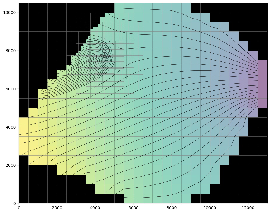
Plot heads and particle paths over the grid.
[12]:
fig = plt.figure(figsize=(11, 11))
ax = fig.add_subplot(1, 1, 1, aspect="equal")
mm = flopy.plot.PlotMapView(model=gwf)
mm.plot_grid(lw=0.5, alpha=0.5)
mm.plot_ibound()
mm.plot_array(hd, alpha=0.5)
mm.plot_pathline(pl, layer="all", lw=0.3, colors=["black"])
plt.show()
Clean up the temporary workspace.
[13]:
try:
    # ignore PermissionError on Windows
    temp_dir.cleanup()
except:
    pass