Working with MODPATH 6
This notebook demonstrates forward and backward tracking with MODPATH. The notebook also shows how to create subsets of pathline and endpoint information, plot MODPATH results on ModelMap objects, and export endpoints and pathlines as shapefiles.
[1]:
import os
import shutil
[2]:
import sys
from pprint import pformat
from tempfile import TemporaryDirectory

import git
import matplotlib as mpl
import matplotlib.pyplot as plt
import numpy as np
import pandas as pd
import pooch

import flopy

print(sys.version)
print(f"numpy version: {np.__version__}")
print(f"matplotlib version: {mpl.__version__}")
print(f"pandas version: {pd.__version__}")
print(f"flopy version: {flopy.__version__}")
3.10.18 | packaged by conda-forge | (main, Jun  4 2025, 14:45:41) [GCC 13.3.0]
numpy version: 2.2.6
matplotlib version: 3.10.6
pandas version: 2.3.3
flopy version: 3.11.0.dev0
Load the MODFLOW model, then switch to a temporary working directory.
[3]:
from pathlib import Path

# Check if we are in the repository and define the data path.

try:
    root = Path(git.Repo(".", search_parent_directories=True).working_dir)
except:
    root = None

data_path = root / "examples" / "data" if root else Path.cwd()

# temporary directory
temp_dir = TemporaryDirectory()
model_ws = Path(temp_dir.name)

file_names = {
    "EXAMPLE-1.endpoint": None,
    "EXAMPLE-1.mpsim": None,
    "EXAMPLE-2.endpoint": None,
    "EXAMPLE-2.mplist": None,
    "EXAMPLE-2.mpsim": None,
    "EXAMPLE-3.endpoint": None,
    "EXAMPLE-3.mplist": None,
    "EXAMPLE-3.mpsim": None,
    "EXAMPLE-3.pathline": None,
    "EXAMPLE-4.endpoint": None,
    "EXAMPLE-4.mplist": None,
    "EXAMPLE-4.mpsim": None,
    "EXAMPLE-4.timeseries": None,
    "EXAMPLE-5.endpoint": None,
    "EXAMPLE-5.mplist": None,
    "EXAMPLE-5.mpsim": None,
    "EXAMPLE-6.endpoint": None,
    "EXAMPLE-6.mplist": None,
    "EXAMPLE-6.mpsim": None,
    "EXAMPLE-6.timeseries": None,
    "EXAMPLE-7.endpoint": None,
    "EXAMPLE-7.mplist": None,
    "EXAMPLE-7.mpsim": None,
    "EXAMPLE-7.timeseries": None,
    "EXAMPLE-8.endpoint": None,
    "EXAMPLE-8.mplist": None,
    "EXAMPLE-8.mpsim": None,
    "EXAMPLE-8.timeseries": None,
    "EXAMPLE-9.endpoint": None,
    "EXAMPLE-9.mplist": None,
    "EXAMPLE-9.mpsim": None,
    "EXAMPLE.BA6": None,
    "EXAMPLE.BUD": None,
    "EXAMPLE.DIS": None,
    "EXAMPLE.DIS.metadata": None,
    "EXAMPLE.HED": None,
    "EXAMPLE.LPF": None,
    "EXAMPLE.LST": None,
    "EXAMPLE.MPBAS": None,
    "EXAMPLE.OC": None,
    "EXAMPLE.PCG": None,
    "EXAMPLE.RCH": None,
    "EXAMPLE.RIV": None,
    "EXAMPLE.WEL": None,
    "EXAMPLE.mpnam": None,
    "EXAMPLE.nam": None,
    "example-1.mplist": None,
    "example-6.locations": None,
    "example-7.locations": None,
    "example-8.locations": None,
    "example.basemap": None,
}
for fname, fhash in file_names.items():
    pooch.retrieve(
        url=f"https://github.com/modflowpy/flopy/raw/develop/examples/data/mp6/{fname}",
        fname=fname,
        path=data_path / "mp6",
        known_hash=fhash,
    )

shutil.copytree(data_path / "mp6", model_ws, dirs_exist_ok=True)

mffiles = list(model_ws.glob("EXAMPLE.*"))

m = flopy.modflow.Modflow.load("EXAMPLE.nam", model_ws=model_ws)

hdsfile = flopy.utils.HeadFile(os.path.join(model_ws, "EXAMPLE.HED"))
hdsfile.get_kstpkper()

hds = hdsfile.get_data(kstpkper=(0, 2))
Plot RIV bc and head results.
[4]:
plt.imshow(hds[4, :, :])
plt.colorbar()
[4]:
<matplotlib.colorbar.Colorbar at 0x7fde23fd7be0>

[5]:
fig = plt.figure(figsize=(8, 8))
ax = fig.add_subplot(1, 1, 1, aspect="equal")
mapview = flopy.plot.PlotMapView(model=m, layer=4)
quadmesh = mapview.plot_ibound()
linecollection = mapview.plot_grid()
riv = mapview.plot_bc("RIV", color="g", plotAll=True)
quadmesh = mapview.plot_bc("WEL", kper=1, plotAll=True)
contour_set = mapview.contour_array(
    hds, levels=np.arange(np.min(hds), np.max(hds), 0.5), colors="b"
)
plt.clabel(contour_set, inline=1, fontsize=14)
[5]:
<a list of 5 text.Text objects>

Now create forward particle tracking simulation where particles are released at the top of each cell in layer 1:
specifying the recharge package in
create_mpsimreleases a single particle on iface=6 of each top cellstart the particles at begining of per 3, step 1, as in example 3 in MODPATH6 manual
Note: in FloPy version 3.3.5 and previous, the Modpath6 constructor dis_file, head_file and budget_file arguments expected filenames relative to the model workspace. In 3.3.6 and later, full paths must be provided — if they are not, discretization, head and budget data are read directly from the model, as before.
[6]:
from os.path import join

mp = flopy.modpath.Modpath6(
    modelname="ex6",
    exe_name="mp6",
    modflowmodel=m,
    model_ws=str(model_ws),
)

mpb = flopy.modpath.Modpath6Bas(
    mp, hdry=m.lpf.hdry, laytyp=m.lpf.laytyp, ibound=1, prsity=0.1
)

# start the particles at begining of per 3, step 1, as in example 3 in MODPATH6 manual
# (otherwise particles will all go to river)
sim = mp.create_mpsim(
    trackdir="forward",
    simtype="pathline",
    packages="RCH",
    start_time=(2, 0, 1.0),
)

mp.change_model_ws(model_ws)
mp.write_name_file()
mp.write_input()
success, buff = mp.run_model(silent=True, report=True)
assert success, pformat(buff)
Read in the endpoint file and plot particles that terminated in the well.
[7]:
fpth = os.path.join(model_ws, "ex6.mpend")
epobj = flopy.utils.EndpointFile(fpth)
well_epd = epobj.get_destination_endpoint_data(dest_cells=[(4, 12, 12)])
# returns record array of same form as epobj.get_all_data()
[8]:
well_epd[0:2]
[8]:
rec.array([(50, 0, 2, 0., 29565.62, 1, 0, 2, 0, 6, 0, 0.5, 0.5, 1., 200., 9000., 339.1231, 1, 4, 12, 12, 2, 0, 1.       , 0.9178849, 0.09755219, 5200.   , 5167.154,  9.755219, b'rch'),
           (75, 0, 2, 0., 26106.59, 1, 0, 3, 0, 6, 0, 0.5, 0.5, 1., 200., 8600., 339.1203, 1, 4, 12, 12, 4, 0, 0.7848778, 1.       , 0.1387314 , 5113.951, 5200.   , 13.87314 , b'rch')],
          dtype=[('particleid', '<i4'), ('particlegroup', '<i4'), ('status', '<i4'), ('time0', '<f4'), ('time', '<f4'), ('initialgrid', '<i4'), ('k0', '<i4'), ('i0', '<i4'), ('j0', '<i4'), ('cellface0', '<i4'), ('zone0', '<i4'), ('xloc0', '<f4'), ('yloc0', '<f4'), ('zloc0', '<f4'), ('x0', '<f4'), ('y0', '<f4'), ('z0', '<f4'), ('finalgrid', '<i4'), ('k', '<i4'), ('i', '<i4'), ('j', '<i4'), ('cellface', '<i4'), ('zone', '<i4'), ('xloc', '<f4'), ('yloc', '<f4'), ('zloc', '<f4'), ('x', '<f4'), ('y', '<f4'), ('z', '<f4'), ('label', 'O')])
[9]:
fig = plt.figure(figsize=(8, 8))
ax = fig.add_subplot(1, 1, 1, aspect="equal")
mapview = flopy.plot.PlotMapView(model=m, layer=2)
quadmesh = mapview.plot_ibound()
linecollection = mapview.plot_grid()
riv = mapview.plot_bc("RIV", color="g", plotAll=True)
quadmesh = mapview.plot_bc("WEL", kper=1, plotAll=True)
contour_set = mapview.contour_array(
    hds, levels=np.arange(np.min(hds), np.max(hds), 0.5), colors="b"
)
plt.clabel(contour_set, inline=1, fontsize=14)
mapview.plot_endpoint(well_epd, direction="starting", colorbar=True)
[9]:
<matplotlib.collections.PathCollection at 0x7fde1bb83940>

Write starting locations to a shapefile.
[10]:
fpth = os.path.join(model_ws, "starting_locs.shp")
print(type(fpth))
epobj.write_shapefile(well_epd, direction="starting", shpname=fpth, mg=m.modelgrid)
<class 'str'>
/home/runner/work/flopy/flopy/modflow6/.pixi/envs/rtd/lib/python3.10/site-packages/flopy/utils/modpathfile.py:776: UserWarning: write_shapefile is Deprecated, please use to_geodataframe() in the future
  warnings.warn(
/home/runner/work/flopy/flopy/modflow6/.pixi/envs/rtd/lib/python3.10/site-packages/pyogrio/__init__.py:7: DeprecationWarning: The 'shapely.geos' module is deprecated, and will be removed in a future version. All attributes of 'shapely.geos' are available directly from the top-level 'shapely' namespace (since shapely 2.0.0).
  import shapely.geos  # noqa: F401
/home/runner/work/flopy/flopy/modflow6/.pixi/envs/rtd/lib/python3.10/site-packages/flopy/utils/modpathfile.py:788: UserWarning: Column names longer than 10 characters will be truncated when saved to ESRI Shapefile.
  gdf.to_file(shpname)
/home/runner/work/flopy/flopy/modflow6/.pixi/envs/rtd/lib/python3.10/site-packages/pyogrio/geopandas.py:710: UserWarning: 'crs' was not provided.  The output dataset will not have projection information defined and may not be usable in other systems.
  write(
Read in the pathline file and subset to pathlines that terminated in the well .
[11]:
# make a selection of cells that terminate in the well cell = (4, 12, 12)
pthobj = flopy.utils.PathlineFile(os.path.join(model_ws, "ex6.mppth"))
well_pathlines = pthobj.get_destination_pathline_data(dest_cells=[(4, 12, 12)])
Plot the pathlines that terminate in the well and the starting locations of the particles.
[12]:
fig = plt.figure(figsize=(8, 8))
ax = fig.add_subplot(1, 1, 1, aspect="equal")
mapview = flopy.plot.PlotMapView(model=m, layer=2)
quadmesh = mapview.plot_ibound()
linecollection = mapview.plot_grid()
riv = mapview.plot_bc("RIV", color="g", plotAll=True)
quadmesh = mapview.plot_bc("WEL", kper=1, plotAll=True)
contour_set = mapview.contour_array(
    hds, levels=np.arange(np.min(hds), np.max(hds), 0.5), colors="b"
)
plt.clabel(contour_set, inline=1, fontsize=14)

mapview.plot_endpoint(well_epd, direction="starting", colorbar=True)
# for now, each particle must be plotted individually
# (plot_pathline() will plot a single line for recarray with multiple particles)
# for pid in np.unique(well_pathlines.particleid):
#   modelmap.plot_pathline(pthobj.get_data(pid), layer='all', colors='red');
mapview.plot_pathline(well_pathlines, layer="all", colors="red")
[12]:
<matplotlib.collections.LineCollection at 0x7fde1870f0a0>

Write pathlines to a shapefile.
[13]:
# one line feature per particle
pthobj.write_shapefile(
    well_pathlines,
    direction="starting",
    shpname=os.path.join(model_ws, "pathlines.shp"),
    mg=m.modelgrid,
    verbose=False,
)

# one line feature for each row in pathline file
# (can be used to color lines by time or layer in a GIS)
pthobj.write_shapefile(
    well_pathlines,
    one_per_particle=False,
    shpname=os.path.join(model_ws, "pathlines_1per.shp"),
    mg=m.modelgrid,
    verbose=False,
)
(numpy.record, [('particleid', '<i4'), ('particlegroup', '<i4'), ('timepointindex', '<i4'), ('cumulativetimestep', '<i4'), ('time', '<f4'), ('x', '<f4'), ('y', '<f4'), ('z', '<f4'), ('k', '<i4'), ('i', '<i4'), ('j', '<i4'), ('grid', '<i4'), ('xloc', '<f4'), ('yloc', '<f4'), ('zloc', '<f4'), ('linesegmentindex', '<i4')])
(numpy.record, [('particleid', '<i4'), ('particlegroup', '<i4'), ('timepointindex', '<i4'), ('cumulativetimestep', '<i4'), ('time', '<f4'), ('x', '<f4'), ('y', '<f4'), ('z', '<f4'), ('k', '<i4'), ('i', '<i4'), ('j', '<i4'), ('grid', '<i4'), ('xloc', '<f4'), ('yloc', '<f4'), ('zloc', '<f4'), ('linesegmentindex', '<i4')])
/home/runner/work/flopy/flopy/modflow6/.pixi/envs/rtd/lib/python3.10/site-packages/flopy/utils/particletrackfile.py:353: DeprecationWarning: write_shapefile will be Deprecated, please use to_geo_dataframe()
  warnings.warn(
/home/runner/work/flopy/flopy/modflow6/.pixi/envs/rtd/lib/python3.10/site-packages/flopy/utils/particletrackfile.py:369: UserWarning: Column names longer than 10 characters will be truncated when saved to ESRI Shapefile.
  gdf.to_file(shpname)
/home/runner/work/flopy/flopy/modflow6/.pixi/envs/rtd/lib/python3.10/site-packages/pyogrio/geopandas.py:710: UserWarning: 'crs' was not provided.  The output dataset will not have projection information defined and may not be usable in other systems.
  write(
Replace WEL package with MNW2, and create backward tracking simulation using particles released at MNW well.
[14]:
m2 = flopy.modflow.Modflow.load(
    "EXAMPLE.nam", model_ws=str(model_ws), exe_name="mf2005"
)
m2.get_package_list()
[14]:
['DIS', 'BAS6', 'WEL', 'RIV', 'RCH', 'OC', 'PCG', 'LPF']
[15]:
m2.nrow_ncol_nlay_nper
[15]:
(25, 25, 5, 3)
[16]:
m2.wel.stress_period_data.data
[16]:
{0: 0,
 1: rec.array([(4, 12, 12, -150000., 0.)],
           dtype=[('k', '<i8'), ('i', '<i8'), ('j', '<i8'), ('flux', '<f4'), ('iface', '<f4')]),
 2: rec.array([(4, 12, 12, -150000., 0.)],
           dtype=[('k', '<i8'), ('i', '<i8'), ('j', '<i8'), ('flux', '<f4'), ('iface', '<f4')])}
[17]:
node_data = np.array(
    [
        (3, 12, 12, "well1", "skin", -1, 0, 0, 0, 1.0, 2.0, 5.0, 6.2),
        (4, 12, 12, "well1", "skin", -1, 0, 0, 0, 0.5, 2.0, 5.0, 6.2),
    ],
    dtype=[
        ("k", int),
        ("i", int),
        ("j", int),
        ("wellid", object),
        ("losstype", object),
        ("pumploc", int),
        ("qlimit", int),
        ("ppflag", int),
        ("pumpcap", int),
        ("rw", float),
        ("rskin", float),
        ("kskin", float),
        ("zpump", float),
    ],
).view(np.recarray)

stress_period_data = {
    0: np.array(
        [(0, "well1", -150000.0)],
        dtype=[("per", int), ("wellid", object), ("qdes", float)],
    )
}
[18]:
m2.name = "Example_mnw"
m2.remove_package("WEL")
mnw2 = flopy.modflow.ModflowMnw2(
    model=m2,
    mnwmax=1,
    node_data=node_data,
    stress_period_data=stress_period_data,
    itmp=[1, -1, -1],
)
m2.get_package_list()
[18]:
['DIS', 'BAS6', 'RIV', 'RCH', 'OC', 'PCG', 'LPF', 'MNW2']
Write and run MODFLOW.
[19]:
m2.change_model_ws(model_ws)
m2.write_name_file()
m2.write_input()
success, buff = m2.run_model(silent=True, report=True)
assert success, pformat(buff)
Create a new Modpath6 object.
[20]:
mp = flopy.modpath.Modpath6(
    modelname="ex6mnw",
    exe_name="mp6",
    modflowmodel=m2,
    model_ws=model_ws,
)

mpb = flopy.modpath.Modpath6Bas(
    mp, hdry=m2.lpf.hdry, laytyp=m2.lpf.laytyp, ibound=1, prsity=0.1
)
sim = mp.create_mpsim(trackdir="backward", simtype="pathline", packages="MNW2")

mp.change_model_ws(model_ws)
mp.write_name_file()
mp.write_input()
success, buff = mp.run_model(silent=True, report=True)
if success:
    for line in buff:
        print(line)
else:
    raise ValueError("Failed to run.")
Processing basic data ...
Checking head file ...
Checking budget file and building index ...

Run particle tracking simulation ...
Processing Time Step     1 Period     1.  Time =  2.00000E+05
Particle tracking complete. Writing endpoint file ...
End of MODPATH simulation. Normal termination.
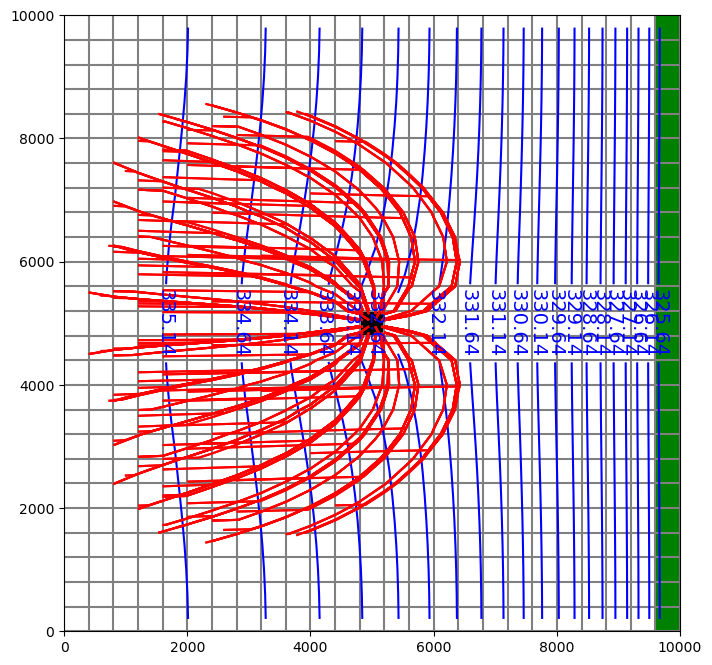
Read in results and plot.
[21]:
pthobj = flopy.utils.PathlineFile(os.path.join(model_ws, "ex6mnw.mppth"))
epdobj = flopy.utils.EndpointFile(os.path.join(model_ws, "ex6mnw.mpend"))
well_epd = epdobj.get_alldata()
well_pathlines = pthobj.get_alldata()  # returns a list of recarrays; one per pathline
[22]:
fig = plt.figure(figsize=(8, 8))
ax = fig.add_subplot(1, 1, 1, aspect="equal")
mapview = flopy.plot.PlotMapView(model=m2, layer=2)
quadmesh = mapview.plot_ibound()
linecollection = mapview.plot_grid()
riv = mapview.plot_bc("RIV", color="g", plotAll=True)
quadmesh = mapview.plot_bc("MNW2", kper=1, plotAll=True)
contour_set = mapview.contour_array(
    hds, levels=np.arange(np.min(hds), np.max(hds), 0.5), colors="b"
)
plt.clabel(contour_set, inline=1, fontsize=14)

mapview.plot_pathline(well_pathlines, travel_time="<10000", layer="all", colors="red")
[22]:
<matplotlib.collections.LineCollection at 0x7fde117e08b0>
[23]:
try:
    # ignore PermissionError on Windows
    temp_dir.cleanup()
except:
    pass