Advection, Dispersion and Decay in a One-Dimensional Uniform Flow Field
Panday, S., 2024; USG-Transport Version 2.4.0: Transport and Other Enhancements to MODFLOW-USG, GSI Environmental, July 2024 http://www.gsi-net.com/en/software/free-software/USG-Transport.html
This test problem discusses one dimensional advective dispersive transport with first-order decay of a chemical species, from a prescribed concentration source in a uniform, steady-state flow field. A 1000-foot-long domain is discretized into 2 layers, 2 rows, and 101 columns using ∆x =∆y = 10 feet, and ∆z = 5 feet. Two layers and rows were selected for convenience. The flow-field is setup using a hydraulic conductivity of 10 ft/day and constant head boundaries of 1,100 feet and 100 feet at either end of the domain. The seepage velocity is thus v = 50 feet/day, for an effective porosity of 0.2.
Transport simulations were performed for 20 days using 1000 time-steps of fixed size ∆t = 0.2 days. Initial concentration of water within the domain was zero, and a prescribed concentration of 1 mg/L was set at the upstream end of the domain for the duration of the simulation.
[1]:
import matplotlib.pyplot as plt
import numpy as np

import flopy
from flopy.mfusg import MfUsg, MfUsgBas, MfUsgBct, MfUsgLpf, MfUsgOc, MfUsgPcb, MfUsgSms
from flopy.modflow import ModflowDis
from flopy.utils import HeadFile
[2]:
model_ws = "Ex1_1D"
mf = MfUsg(
    version="mfusg",
    structured=True,
    model_ws=model_ws,
    modelname="ex1-1d",
    exe_name="mfusg_gsi",
)
[3]:
nlay = 2
nrow = 2
ncol = 101
delr = 10
delc = 10
top = 10
botm = [5, 0]
perlen = 20
nstp = 1000
lenuni = 0

xcol = [i * delc for i in range(ncol)]

dis = ModflowDis(
    mf,
    nlay=nlay,
    nrow=nrow,
    ncol=ncol,
    delr=delr,
    delc=delc,
    top=top,
    botm=botm,
    perlen=perlen,
    nstp=nstp,
    lenuni=lenuni,
)
[4]:
ibound = np.ones((nlay, nrow, ncol))
ibound[:, :, 0] = -1
ibound[:, :, -1] = -1

strt = np.full((nlay, nrow, ncol), 100.0)
strt[:, :, 0] = 1100.0

bas = MfUsgBas(mf, ibound=ibound, strt=strt)
[5]:
ipakcb = 50
hk = 10.0
vka = 10.0

lpf = MfUsgLpf(mf, ipakcb=ipakcb, laytyp=3, hk=hk, vka=vka)
[6]:
sms = MfUsgSms(
    mf,
    hclose=5e-2,
    hiclose=1e-5,
    mxiter=250,
    iter1=600,
    iprsms=1,
    nonlinmeth=2,
    linmeth=1,
    theta=0.7,
    akappa=0.07,
    gamma=0.1,
    amomentum=0.0,
    numtrack=200,
    btol=1.1,
    breduc=0.2,
    reslim=1.0,
    iacl=2,
    norder=0,
    level=7,
    north=14,
    iredsys=0,
    rrctol=0.0,
    idroptol=1,
    epsrn=1.0e-3,
)
[7]:
lrcsc = []
for ilay in range(nlay):
    for irow in range(nrow):
        lrcsc.append([ilay, irow, 0, 1, 1.0])  # inlet
        lrcsc.append([ilay, irow, ncol - 1, 1, 0.0])  # outlet
pcb = MfUsgPcb(mf, stress_period_data={0: lrcsc})
[8]:
oc = MfUsgOc(
    mf,
    save_conc=1,
    save_every=1,
    save_types=["save head", "save budget"],
    unitnumber=[14, 30, 31, 0, 0, 33],
)
Case 1 conducts the simulation with zero dispersion.
[9]:
prsity = 0.2
dl = 0
dt = 0
conc = 0
bct = MfUsgBct(
    mf,
    ipakcb=55,
    itvd=4,
    cinact=-999.0,
    diffnc=0.0,
    prsity=prsity,
    dl=dl,
    dt=dt,
    conc=conc,
)
[10]:
mf.write_input()
success, buff = mf.run_model(silent=True)
True
[11]:
concobj = HeadFile(f"{mf.model_ws}/{mf.name}.con", text="conc")
# Get the cocentration data at 10 days
conc_case1 = concobj.get_data(totim=10.0)[0, 0, :]
[12]:
mf.remove_package("BCT")
bct = MfUsgBct(
    mf,
    ipakcb=55,
    itvd=0,
    cinact=-999.0,
    diffnc=0.0,
    prsity=prsity,
    dl=dl,
    dt=dt,
    conc=conc,
)
mf.write_input()
success, buff = mf.run_model(silent=True)
True
[13]:
concobj = HeadFile(f"{mf.model_ws}/{mf.name}.con", text="conc")
# Get the cocentration data at 10 days
conc_case1_ups = concobj.get_data(totim=10.0)[0, 0, :]
[14]:
mf.remove_package("BCT")
bct = MfUsgBct(
    mf,
    ipakcb=55,
    itvd=0,
    timeweight=0.0,
    cinact=-999.0,
    diffnc=0.0,
    prsity=prsity,
    dl=dl,
    dt=dt,
    conc=conc,
)
mf.write_input()
success, buff = mf.run_model(silent=True)
True
[15]:
concobj = HeadFile(f"{mf.model_ws}/{mf.name}.con", text="conc")
# Get the cocentration data at 10 days
conc_case1_cn = concobj.get_data(totim=10.0)[0, 0, :]
[16]:
analytical = np.ones(ncol)
analytical[50] = 0.5
analytical[51:] = 0.0
Case 2 includes a retardation of 2 by using a bulk density value of 1 kg/L and an adsorption coefficient (kd) of 0.2 L/kg.
[17]:
mf.remove_package("BCT")
bulkd = 1
adsorb = 0.2
bct = MfUsgBct(
    mf,
    ipakcb=55,
    itvd=4,
    cinact=-999.0,
    diffnc=0.0,
    prsity=prsity,
    iadsorb=1,
    bulkd=bulkd,
    adsorb=adsorb,
    dl=dl,
    dt=dt,
    conc=conc,
)
[18]:
mf.write_input()
success, buff = mf.run_model(silent=True)
True
[19]:
concobj = HeadFile(f"{mf.model_ws}/{mf.name}.con", text="conc")
# Get the cocentration data at 10 days
conc_case2 = concobj.get_data(totim=20.0)[0, 0, :]
[20]:
fig = plt.figure(figsize=(8, 5), dpi=150)
ax = fig.add_subplot(111)
ax.plot(xcol, conc_case1, label="case 1 TVD 10d")
ax.plot(xcol, analytical, label="analytical solution 10d")
ax.plot(xcol, conc_case1_ups, label="case 1 Upstream 10d")
ax.plot(xcol, conc_case1_cn, label="case 1 Crank-Nicolson 10d")
ax.plot(xcol, conc_case2, label="case 2  20d")
ax.set_xlabel("Distance (feet)")
ax.set_ylabel("Normalized concentration")
ax.set_title(
    "MODFLOW-USG Transport Simulation Results for Advection in a One-Dimensional, Uniform Flow Field"
)

ax.legend()
[20]:
<matplotlib.legend.Legend at 0x7ff3c6dbe060>
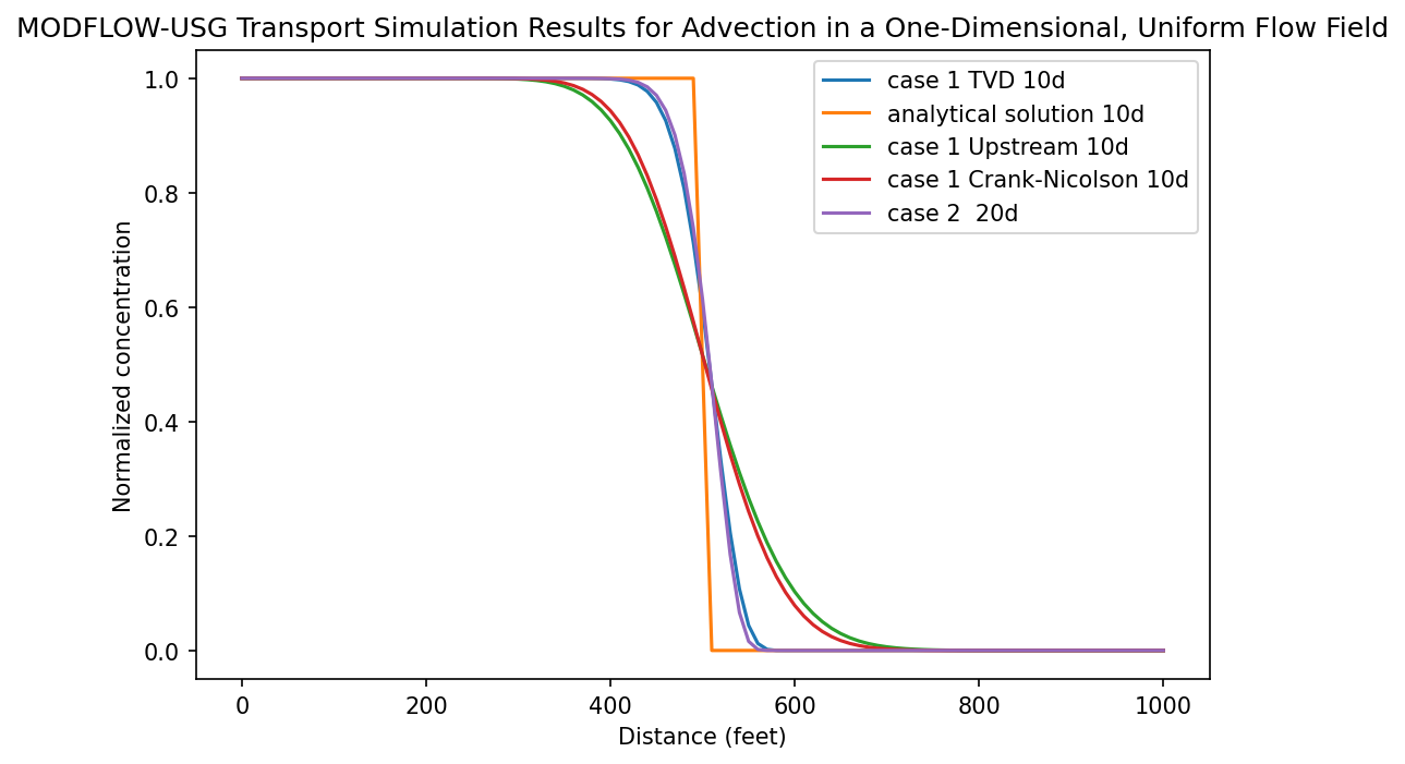
Figure Ex 1 shows the simulation results after 10 days of simulation, when the advective front of Case 1 moves halfway into the one-dimensional domain. Results are presented for an upstream weighted solution and for a solution using the TVD scheme with 4 TVD iterations. The purely advective analytical solution is also shown on the figure for comparison. It is noted that the TVD scheme greatly reduces numerical dispersion associated with the upstream weighted scheme; the sharp front is resolved over a span of 11 grid-blocks with the TVD scheme, as compared to about 32 grid-blocks with the upstream weighted scheme. However, this too may be considered too numerically dispersed for an advective solution involving non-linear reactive transport (where the reactions dominate only in the dilute fringes of the plume) and therefore a finer discretization should be provided in regions where a sharp advective front may be encountered and where such accuracy is important. Figure Ex 1 also shows the simulation results after 20 days of simulation for Case 2 using 4 TVD iterations. With a retardation of 2, this front is noted to move the same amount in 20 days as for Case 1 in 10 days.
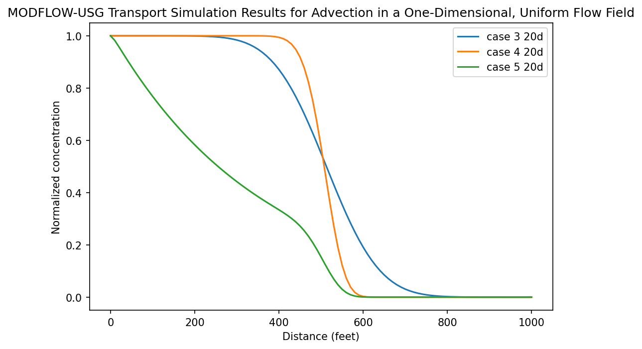
Case 3 further includes a longitudinal dispersivity value of 10 feet (grid Peclet number of 1)
[21]:
mf.remove_package("BCT")
dl = 10.0

bct = MfUsgBct(
    mf,
    ipakcb=55,
    itvd=4,
    cinact=-999.0,
    diffnc=0.0,
    prsity=prsity,
    iadsorb=1,
    bulkd=bulkd,
    adsorb=adsorb,
    dl=dl,
    dt=dt,
    conc=conc,
)
[22]:
mf.write_input()
success, buff = mf.run_model(silent=True)
True
[23]:
concobj = HeadFile(f"{mf.model_ws}/{mf.name}.con", text="conc")
# Get the cocentration data at 10 days
conc_case3 = concobj.get_data(totim=20.0)[0, 0, :]
Case 4 includes a longitudinal dispersivity value of 1 feet (grid Peclet Number of 10)
[24]:
mf.remove_package("BCT")
dl = 1.0

bct = MfUsgBct(
    mf,
    ipakcb=55,
    itvd=4,
    cinact=-999.0,
    diffnc=0.0,
    prsity=prsity,
    iadsorb=1,
    bulkd=bulkd,
    adsorb=adsorb,
    dl=dl,
    dt=dt,
    conc=conc,
)
[25]:
mf.write_input()
success, buff = mf.run_model(silent=True)
True
[26]:
concobj = HeadFile(f"{mf.model_ws}/{mf.name}.con", text="conc")
# Get the cocentration data at 10 days
conc_case4 = concobj.get_data(totim=20.0)[0, 0, :]
Case 5 also includes first order decay with a half-life of 10 days (first order decay rate of 6.9315x 10⁻² /day) on the simulation with the high grid Peclet Number.
[27]:
mf.remove_package("BCT")
fodrw = 6.9315e-2
fodrs = 6.9315e-2

bct = MfUsgBct(
    mf,
    ipakcb=55,
    itvd=4,
    cinact=-999.0,
    diffnc=0.0,
    prsity=prsity,
    iadsorb=1,
    bulkd=bulkd,
    adsorb=adsorb,
    ifod=3,
    fodrw=fodrw,
    fodrs=fodrs,
    dl=dl,
    dt=dt,
    conc=conc,
)
[28]:
mf.write_input()
success, buff = mf.run_model(silent=True)
True
[29]:
concobj = HeadFile(f"{mf.model_ws}/{mf.name}.con", text="conc")
# Get the cocentration data at 10 days
conc_case5 = concobj.get_data(totim=20.0)[0, 0, :]
[30]:
# Results for the simulation cases 3, 4 and 5 are shown on Figure Ex 2 along with analytical solution results for the respective cases at 20 days. The Domenico spreadsheet analytical solution was used for comparison (www.elibrary.dep.state.pa.us/dsweb/Get/Version49262/ Quick_Domenico.xls). The simulation results for all three cases are almost the same as the respective analytical solution results. The largest errors occurred for Case 4 with a high Peclet number of 10, however, inclusion of decay diminished that error as noted for Case 5. Thus, it is noted that solution accuracy of advective transport improves substantially if a reasonable amount of dispersion or solute decay is present. Numerical experiments with different numbers of TVD iterations (including use of just two iterations as in a predictor/corrector approach) did not noticeably change the results for any of the cases discussed above.
#
[31]:
fig = plt.figure(figsize=(8, 5), dpi=150)
ax = fig.add_subplot(111)
ax.plot(xcol, conc_case3, label="case 3 20d")
ax.plot(xcol, conc_case4, label="case 4 20d")
ax.plot(xcol, conc_case5, label="case 5 20d")
ax.set_xlabel("Distance (feet)")
ax.set_ylabel("Normalized concentration")
ax.set_title(
    "MODFLOW-USG Transport Simulation Results for Advection in a One-Dimensional, Uniform Flow Field"
)

ax.legend()
[31]:
<matplotlib.legend.Legend at 0x7ff3c6b23380>