Advection and Dispersion in a Two-Dimensional Confined Radial Flow Field
Panday, S., 2024; USG-Transport Version 2.4.0: Transport and Other Enhancements to MODFLOW-USG, GSI Environmental, July 2024 http://www.gsi-net.com/en/software/free-software/USG-Transport.html
This test problem discusses advective dispersive transport of a chemical species in a radial flow field resulting from injection of a dissolved chemical species at the center of a 10,000 feet by 10,000 feet square simulation domain. The domain is discretized into 1 layer, 100 rows, and 100 columns with grid size of 100x100 feet, and thickness of 15feet. A confined flow-field is setup using a hydraulic conductivity of 100 ft/day, a constant head boundary condition of 20 feet around the perimeter, and a well at row = 50 and column = 50, that injects fluid at a rate of 10,000 ft3/day. The concentration of water in the domain is zero at the start of the simulation. The species concentration in injected water is 1mg/L. The dispersivity values used were 500 feet and 50 feet for the longitudinal and transverse directions respectively, and the effective porosity value used was 0.2. The transport simulation was conducted for 5,000 days with 50 time steps using a fixed time step size of 100 days. Also, the cross-dispersion option was activated. Simulation results for this test case are compared with results from an MT3D (Zheng and Wang, 1999) simulation with an identical setup.
[1]:
import matplotlib.pyplot as plt
import numpy as np

import flopy
from flopy.mfusg import MfUsg, MfUsgBas, MfUsgBct, MfUsgLpf, MfUsgOc, MfUsgSms, MfUsgWel
from flopy.modflow import ModflowChd, ModflowDis
from flopy.utils import HeadFile
[2]:
model_ws = "Ex2_Radial"
mf = MfUsg(
    version="mfusg",
    structured=True,
    model_ws=model_ws,
    modelname="Ex2_Radial",
    exe_name="mfusg_gsi",
)
[3]:
nlay = 1
nrow = 100
ncol = 100
delr = 100.0
delc = 100.0
top = 15
botm = 0

perlen = 5000.0
nstp = 50
lenuni = 0

xcol = [i * delc for i in range(ncol)]

dis = ModflowDis(
    mf,
    nlay=nlay,
    nrow=nrow,
    ncol=ncol,
    delr=delr,
    delc=delc,
    top=top,
    botm=botm,
    perlen=perlen,
    nstp=nstp,
    lenuni=lenuni,
)
[4]:
ibound = np.ones((nlay, nrow, ncol))
ibound[:, 0, :] = -1
ibound[:, -1, :] = -1
ibound[:, :, 0] = -1
ibound[:, :, -1] = -1

strt = np.full((nlay, nrow, ncol), 15.0)
strt[:, 0, :] = 20.0
strt[:, -1, :] = 20.0
strt[:, :, 0] = 20.0
strt[:, :, -1] = 20.0

bas = MfUsgBas(mf, ibound=ibound, strt=strt)
[5]:
ipakcb = 50
hk = 100.0
vka = 100.0

lpf = MfUsgLpf(mf, ipakcb=ipakcb, laytyp=1, hk=hk, vka=vka)
[6]:
sms = MfUsgSms(
    mf,
    hclose=1.0e-3,
    hiclose=1.0e-5,
    mxiter=220,
    iter1=600,
    iprsms=1,
    nonlinmeth=2,
    linmeth=1,
    theta=0.9,
    akappa=0.07,
    gamma=0.1,
    amomentum=0.0,
    numtrack=200,
    btol=1.1,
    breduc=0.2,
    reslim=1.0,
    iacl=2,
    norder=1,
    level=3,
    north=14,
    iredsys=0,
    rrctol=0.0,
    idroptol=0,
    epsrn=1.0e-3,
)
[7]:
lrcsc = []
for icol in range(ncol):
    lrcsc.append([0, 0, icol, 20.0, 20.0])
for irow in range(1, nrow - 1):
    lrcsc.append([0, irow, 0, 20.0, 20.0])
    lrcsc.append([0, irow, 99, 20.0, 20.0])
for icol in range(ncol):
    lrcsc.append([0, 99, icol, 20.0, 20.0])

chd = ModflowChd(mf, stress_period_data={0: lrcsc})
[8]:
lrcsc = {0: [0, 49, 49, 10000.000, 1.0, 1.0]}
dtype = np.dtype(
    [
        ("k", int),
        ("i", int),
        ("j", int),
        ("flux", np.float32),
        ("con1", np.float32),
        ("c01", np.float32),
    ]
)
wel = MfUsgWel(mf, ipakcb=ipakcb, options=[], dtype=dtype, stress_period_data=lrcsc)
[9]:
oc = MfUsgOc(
    mf,
    save_conc=1,
    save_every=1,
    save_types=["save head", "save budget"],
    unitnumber=[14, 30, 31, 0, 0, 33],
)
Advection
[10]:
prsity = 0.2
dl = 0
dt = 0
conc = 0
bct = MfUsgBct(
    mf,
    ipakcb=55,
    itvd=4,
    cinact=-999.0,
    diffnc=0.0,
    prsity=prsity,
    dl=dl,
    dt=dt,
    conc=conc,
)
[11]:
mf.write_input()
success, buff = mf.run_model(silent=True)
True
[12]:
concobj = HeadFile(f"{mf.model_ws}/{mf.name}.con", text="conc")
conc_adv = concobj.get_data(totim=5000.0)[0]
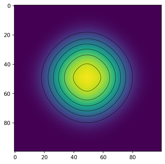
[13]:
fig = plt.figure(figsize=(8, 5), dpi=150)
ax = fig.add_subplot(111)
im = ax.imshow(conc_adv, vmin=conc_adv.min(), vmax=conc_adv.max())
ctr = ax.contour(conc_adv, colors="k", linewidths=0.5)
[14]:
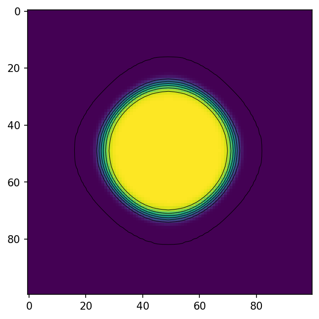
# ### Dispersion - without cross disperion
[15]:
mf.remove_package("BCT")
dl = 500.0
dt = 50.0
bct = MfUsgBct(
    mf,
    ipakcb=55,
    itvd=8,
    cinact=-999.0,
    diffnc=0.0,
    prsity=prsity,
    dl=dl,
    dt=dt,
    conc=conc,
)
[16]:
mf.write_input()
success, buff = mf.run_model(silent=True)
True
[17]:
concobj = HeadFile(f"{mf.model_ws}/{mf.name}.con", text="conc")
conc_disp = concobj.get_data(totim=5000.0)[0]
[18]:
fig = plt.figure(figsize=(8, 5), dpi=150)
ax = fig.add_subplot(111)
im = ax.imshow(conc_disp, vmin=conc_adv.min(), vmax=conc_adv.max())
ctr = ax.contour(conc_disp, colors="k", linewidths=0.5)
[19]:
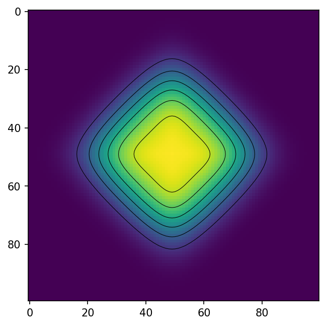
# ### Dispersion - with cross disperion
[20]:
mf.remove_package("BCT")
bct = MfUsgBct(
    mf,
    ipakcb=55,
    itvd=8,
    cinact=-999.0,
    diffnc=0.0,
    ixdisp=1,
    prsity=prsity,
    dl=dl,
    dt=dt,
    conc=conc,
)
[21]:
mf.write_input()
success, buff = mf.run_model(silent=True)
True
[22]:
concobj = HeadFile(f"{mf.model_ws}/{mf.name}.con", text="conc")
conc_xdisp = concobj.get_data(totim=5000.0)[0]
[23]:
fig = plt.figure(figsize=(8, 5), dpi=150)
ax = fig.add_subplot(111)
im = ax.imshow(conc_xdisp, vmin=conc_adv.min(), vmax=conc_adv.max())
ctr = ax.contour(conc_xdisp, colors="k", linewidths=0.5)