This page was generated from mfusg_transport_tutorial06_StallmanHeatTransport.py. It's also available as a notebook.

MF-USG Verification Example for Heat and Solute Transport - Ex6 Stallman

Panday, S., 2024; USG-Transport Version 2.4.0: Transport and Other Enhancements to MODFLOW-USG, GSI Environmental, July 2024 http://www.gsi-net.com/en/software/free-software/USG-Transport.html

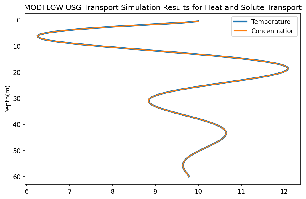
The problem compares the MODFLOW-USG solution with the Stallman (1965) analytical solution for transient heat flow in the subsurface in response to a sinusoidally varying temperature boundary at land surface. The transport model is simulated with both heat and equivalent solute conditions. The heat transport parameters and equivalent solute parameters are shown on Table H1 below.

import os

import matplotlib.pyplot as plt
import numpy as np

import flopy
from flopy.mfusg import (
    MfUsg,
    MfUsgBas,
    MfUsgBct,
    MfUsgDdf,
    MfUsgDisU,
    MfUsgLpf,
    MfUsgOc,
    MfUsgPcb,
    MfUsgSms,
    MfUsgWel,
)
from flopy.modflow import ModflowChd, ModflowDis
from flopy.plot import PlotCrossSection
from flopy.utils import HeadUFile
from flopy.utils.gridgen import Gridgen

model_ws = "Ex6a_Stallman_Heat"
mf = MfUsg(
    version="mfusg",
    structured=False,
    model_ws=model_ws,
    modelname="Ex6_Stallman",
    exe_name="mfusg_gsi",
)

# The problem consists of a saturated vertical soil column 60 m long discretized in to 120 cells with a uniform thickness of 0.5 m each.
ms = flopy.modflow.Modflow()

nrow = 1
ncol = 1
delc = 1.0
delr = 1.0

nlay = 120
delv = 0.5
top = 60.0
botm = np.linspace(top - delv, 0.0, nlay)

dis = flopy.modflow.ModflowDis(
    ms, nlay, nrow, ncol, delr=delr, delc=delc, laycbd=0, top=top, botm=botm
)

gridgen_ws = os.path.join(model_ws, "gridgen")
if not os.path.exists(gridgen_ws):
    os.mkdir(gridgen_ws)
g = Gridgen(ms.modelgrid, model_ws=gridgen_ws)
g.build()
gridprops = g.get_gridprops_disu5()

# Number of stress periods: 600;
# Number of time steps in each stress period : 6;
# Simulation time length (s) of each stress period :        525600

nper = 601
perlen = [525600.0] * nper
nstp = [6] * nper
nstp[0] = 1
steady = [False] * nper
steady[0] = True

disu = MfUsgDisU(
    mf, **gridprops, itmuni=1, nper=nper, perlen=perlen, nstp=nstp, steady=steady
)

bas = MfUsgBas(mf, strt=60.0)

# Hydraulic conductivity of 1.0 x 10-4 m/sec (28.35 ft/d). With a porosity of 0.35, the pore velocity is 12.3 cm/d = 1.42 x x 10-6 m/sec.
ipakcb = 50
hk = 1.0e-4
vka = 1.0e-4
ss = 1.0e-10
lpf = MfUsgLpf(
    mf, ipakcb=ipakcb, constantcv=1, novfc=1, laytyp=4, hk=hk, vka=vka, ss=ss
)

sms = MfUsgSms(
    mf,
    hclose=1.0e-3,
    hiclose=1.0e-5,
    mxiter=250,
    iter1=600,
    iprsms=1,
    nonlinmeth=1,
    linmeth=1,
    theta=0.7,
    akappa=0.07,
    gamma=0.1,
    amomentum=0.0,
    numtrack=200,
    btol=1.1,
    breduc=0.2,
    reslim=1.0,
    iacl=1,
    norder=0,
    level=7,
    north=14,
    iredsys=0,
    rrctol=0.0,
    idroptol=1,
    epsrn=1.0e-3,
    options2=["SOLVEACTIVE", "DAMPBOT"],
)

# Downward groundwater flow with a Darcy velocity is of 5 x 10-7 m/sec is generated by a constant head of 60 m at the top and 59.7043 m at the bottom.

# mf.remove_package("CHD")
lrcsc = {}
for iper in range(nper):
    lrcsc[iper] = [[0, 60.0, 60.0], [119, 59.704285, 59.704285]]

chd = ModflowChd(mf, ipakcb=ipakcb, stress_period_data=lrcsc)

Heat Transport

Porosity (unitless) 0.35 Longitudinal dispersivity (m) 0 Transverse dispersivity (m) 0 Diffusion coefficient (ms-1) 1.03E-06 Ambient temperature (oC) 10 Temperature variation (oC) +/- 5 Bulk density (kg/m3) 1709.5

bct = MfUsgBct(
    mf,
    itvd=5,
    idisp=0,
    cinact=-999.9,
    diffnc=0.0,
    timeweight=1.0,
    mcomp=0,
    iheat=1,
    htcondw=0.58,
    rhow=1.0e3,
    htcapw=4.174e3,
    htcaps=800.0,
    htconds=2.0,
    heat=10.0,
    prsity=0.35,
    bulkd=1709.5,
)

# The initial temperature of the subsurface is 10$^\circ$C, and the temperature at the surface varies as $T_{top}=10+5sin(2\pi t/T)$ where t is the time and T is the wave length of 1 year.
simy = (np.cumsum(disu.perlen.array) - perlen) / 3600 / 24 / 365
lrcsc = {}
for iper in range(nper):
    ttop = 10.0 + 5 * np.sin(2 * np.pi * simy[iper])
    lrcsc[iper] = [0, 1, ttop]

pcb = MfUsgPcb(mf, stress_period_data=lrcsc)

oc = MfUsgOc(
    mf,
    save_conc=1,
    save_every=1,
    save_types=["save head", "save budget"],
    unitnumber=[14, 30, 31, 0, 0, 132],
)

mf.write_input()
success, buff = mf.run_model(silent=True)

True

tempobj = HeadUFile(f"{mf.model_ws}/{mf.name}.con", text="tmpr")
simtemp = np.concatenate(tempobj.get_data())

# ## Solute Transport

mf.remove_package("CHD")
dtype = np.dtype(
    [("node", int), ("shead", np.float32), ("ehead", np.float32), ("c01", np.float32)]
)

lrcsc = {}
for iper in range(nper):
    lrcsc[iper] = [[0, 60.0, 60.0, 10.0], [119, 59.704285, 59.704285, 0.0]]

chd = ModflowChd(mf, ipakcb=ipakcb, options=[], dtype=dtype, stress_period_data=lrcsc)

mf.remove_package("BCT")
bct = MfUsgBct(
    mf,
    itvd=5,
    cinact=-999.9,
    diffnc=1.028820e-06,
    nseqitr=1,
    timeweight=1.0,
    prsity=0.35,
    anglex=0.0,
    dl=0.0,
    dt=0.0,
    conc=10.0,
    iadsorb=1,
    bulkd=1709.5,
    adsorb=1.916630e-04,
)

mf.write_input()
success, buff = mf.run_model(silent=True)

True

concobj = HeadUFile(f"{mf.model_ws}/{mf.name}.con", text="conc")
simconc = concobj.get_data()

depth = top - np.squeeze(dis.botm.array)

fig = plt.figure(figsize=(8, 5), dpi=150)
ax = fig.add_subplot(111)
ax.plot(simtemp, depth, label="Temperature", linewidth=3)
ax.plot(simconc, depth, label="Concentration")
plt.gca().invert_yaxis()
ax.set_ylabel("Depth(m)")
ax.set_title("MODFLOW-USG Transport Simulation Results for Heat and Solute Transport")
ax.legend()

<matplotlib.legend.Legend at 0x7fae4d882cc0>

# ## Heat and Solute Transport

mf.remove_package("BCT")
bct = MfUsgBct(
    mf,
    itvd=5,
    cinact=-999.9,
    diffnc=1.028820e-06,
    nseqitr=1,
    timeweight=1.0,
    iheat=1,
    htcondw=0.58,
    rhow=1.0e3,
    htcapw=4.174e3,
    prsity=0.35,
    anglex=0.0,
    dl=0.0,
    dt=0.0,
    conc=10.0,
    iadsorb=1,
    bulkd=1709.5,
    adsorb=1.916630e-04,
    htcaps=800.0,
    htconds=2.0,
    heat=10.0,
)

mf.remove_package("PCB")
simy = (np.cumsum(disu.perlen.array) - perlen) / 3600 / 24 / 365
lrcsc = {}
for iper in range(nper):
    ttop = 10.0 + 5 * np.sin(2 * np.pi * simy[iper])
    lrcsc[iper] = [[0, 1, ttop], [0, 2, ttop]]

pcb = MfUsgPcb(mf, stress_period_data=lrcsc)

mf.write_input()
success, buff = mf.run_model(silent=True)

True

vartype = [
    ("kstp", "<i4"),
    ("kper", "<i4"),
    ("pertim", "<f4"),
    ("totim", "<f4"),
    ("text", "S16"),
    ("nstrt", "<i4"),
    ("nndlay", "<i4"),
    ("ilay", "<i4"),
    ("data", "<f4"),
]
hdr = np.fromfile(f"{mf.model_ws}/{mf.name}.con", vartype)

tmpr_data = hdr[np.char.strip(hdr["text"].astype(str)) == "TMPR"]
conc_data = hdr[np.char.strip(hdr["text"].astype(str)) == "CONC"]
simtemp = tmpr_data[(tmpr_data["kper"] == 601) & (tmpr_data["kstp"] == 6)]["data"]
simconc = conc_data[(conc_data["kper"] == 601) & (conc_data["kstp"] == 6)]["data"]

# tempobj = HeadUFile(f"{mf.model_ws}/{mf.name}.con", precision="single", text=' TMPR           ')
# simtemp = np.concatenate(tempobj.get_data())
#
# concobj = HeadUFile(f"{mf.model_ws}/{mf.name}.con", text="CONC")
# simconc = concobj.get_data()

depth = top - np.squeeze(dis.botm.array)

fig = plt.figure(figsize=(8, 5), dpi=150)
ax = fig.add_subplot(111)
ax.plot(simtemp, depth, label="Temperature", linewidth=3)
ax.plot(simconc, depth, label="Concentration")
plt.gca().invert_yaxis()
ax.set_ylabel("Depth(m)")
ax.set_title("MODFLOW-USG Transport Simulation Results for Heat and Solute Transport")
ax.legend()

<matplotlib.legend.Legend at 0x7fae56c44770>