This page was generated from modflow_postprocessing_example.py. It's also available as a notebook.

Postprocessing head results from MODFLOW

[1]:

import os
import sys
from tempfile import TemporaryDirectory

import matplotlib as mpl
import matplotlib.pyplot as plt
import numpy as np

import flopy
import flopy.utils.binaryfile as bf
from flopy.utils.postprocessing import (
    get_gradients,
    get_transmissivities,
    get_water_table,
)

print(sys.version)
print(f"numpy version: {np.__version__}")
print(f"matplotlib version: {mpl.__version__}")
print(f"flopy version: {flopy.__version__}")

3.12.2 | packaged by conda-forge | (main, Feb 16 2024, 20:50:58) [GCC 12.3.0]
numpy version: 1.26.4
matplotlib version: 3.8.4
flopy version: 3.7.0.dev0

[2]:

mfnam = "EXAMPLE.nam"
model_ws = "../../examples/data/mp6/"
heads_file = "EXAMPLE.HED"

# temporary directory
temp_dir = TemporaryDirectory()
workspace = temp_dir.name

Load example model and head results

[3]:

m = flopy.modflow.Modflow.load(mfnam, model_ws=model_ws)

[4]:

hdsobj = bf.HeadFile(model_ws + heads_file)
hds = hdsobj.get_data(kstpkper=(0, 2))
hds.shape

[4]:

(5, 25, 25)

Plot heads in each layer; export the heads and head contours for viewing in a GIS

for more information about GIS export, type help(export_array), for example

[5]:

fig, axes = plt.subplots(2, 3, figsize=(11, 8.5))
axes = axes.flat
grid = m.modelgrid
for i, hdslayer in enumerate(hds):
    im = axes[i].imshow(hdslayer, vmin=hds.min(), vmax=hds.max())
    axes[i].set_title(f"Layer {i + 1}")
    ctr = axes[i].contour(hdslayer, colors="k", linewidths=0.5)

    # export head rasters
    # (GeoTiff export requires the rasterio package; for ascii grids, just change the extension to *.asc)
    flopy.export.utils.export_array(
        grid, os.path.join(workspace, f"heads{i + 1}.tif"), hdslayer
    )

    # export head contours to a shapefile
    flopy.export.utils.export_array_contours(
        grid, os.path.join(workspace, f"heads{i + 1}.shp"), hdslayer
    )

fig.delaxes(axes[-1])
fig.subplots_adjust(right=0.8)
cbar_ax = fig.add_axes([0.85, 0.15, 0.03, 0.7])
fig.colorbar(im, cax=cbar_ax, label="Head")

No CRS information for writing a .prj file.
Supply an valid coordinate system reference to the attached modelgrid object or .export() method.
No CRS information for writing a .prj file.
Supply an valid coordinate system reference to the attached modelgrid object or .export() method.
No CRS information for writing a .prj file.
Supply an valid coordinate system reference to the attached modelgrid object or .export() method.
No CRS information for writing a .prj file.
Supply an valid coordinate system reference to the attached modelgrid object or .export() method.
No CRS information for writing a .prj file.
Supply an valid coordinate system reference to the attached modelgrid object or .export() method.

[5]:

<matplotlib.colorbar.Colorbar at 0x7f2ebe824620>

../_images/Notebooks_modflow_postprocessing_example_7_2.png

Compare rotated arc-ascii and GeoTiff output

[6]:

grid.set_coord_info(angrot=30.0)
nodata = 0.0
flopy.export.utils.export_array(
    grid, os.path.join(workspace, "heads5_rot.asc"), hdslayer, nodata=nodata
)
flopy.export.utils.export_array(
    grid, os.path.join(workspace, "heads5_rot.tif"), hdslayer, nodata=nodata
)

results = np.loadtxt(os.path.join(workspace, "heads5_rot.asc"), skiprows=6)
results[results == nodata] = np.nan
plt.imshow(results)
plt.colorbar()

[6]:

<matplotlib.colorbar.Colorbar at 0x7f2ebe71b230>

../_images/Notebooks_modflow_postprocessing_example_9_1.png

[7]:

try:
    import rasterio
except:
    rasterio = None
    print("install rasterio to create GeoTiff output")
if rasterio is not None:
    with rasterio.open(os.path.join(workspace, "heads5_rot.tif")) as src:
        print(src.meta)
        plt.imshow(src.read(1))

{'driver': 'GTiff', 'dtype': 'float32', 'nodata': 0.0, 'width': 25, 'height': 25, 'count': 1, 'crs': None, 'transform': Affine(346.4101615137755, 199.99999999999997, -4999.999999999999,
       199.99999999999997, -346.4101615137755, 8660.254037844386)}

../_images/Notebooks_modflow_postprocessing_example_10_1.png

Get the vertical head gradients between layers

[8]:

grad = get_gradients(hds, m, nodata=-999)

fig, axes = plt.subplots(2, 3, figsize=(11, 8.5))
axes = axes.flat

for i, vertical_gradient in enumerate(grad):
    im = axes[i].imshow(vertical_gradient, vmin=grad.min(), vmax=grad.max())
    axes[i].set_title(f"Vertical gradient\nbetween Layers {i + 1} and {i + 2}")
    ctr = axes[i].contour(
        vertical_gradient,
        levels=[-0.1, -0.05, 0.0, 0.05, 0.1],
        colors="k",
        linewidths=0.5,
    )
    plt.clabel(ctr, fontsize=8, inline=1)

fig.delaxes(axes[-2])
fig.delaxes(axes[-1])
fig.subplots_adjust(right=0.8)
cbar_ax = fig.add_axes([0.85, 0.15, 0.03, 0.7])
fig.colorbar(im, cax=cbar_ax, label="positive downward")

[8]:

<matplotlib.colorbar.Colorbar at 0x7f2eadeedee0>

../_images/Notebooks_modflow_postprocessing_example_12_1.png

Get the saturated thickness of a layer

m.modelgrid.saturated_thickness() returns an nlay, nrow, ncol array of saturated thicknesses.

[9]:

st = m.modelgrid.saturated_thickness(hds, mask=-9999.0)

plt.imshow(st[0])
plt.colorbar(label="Saturated thickness")
plt.title("Layer 1")

[9]:

Text(0.5, 1.0, 'Layer 1')

../_images/Notebooks_modflow_postprocessing_example_14_1.png

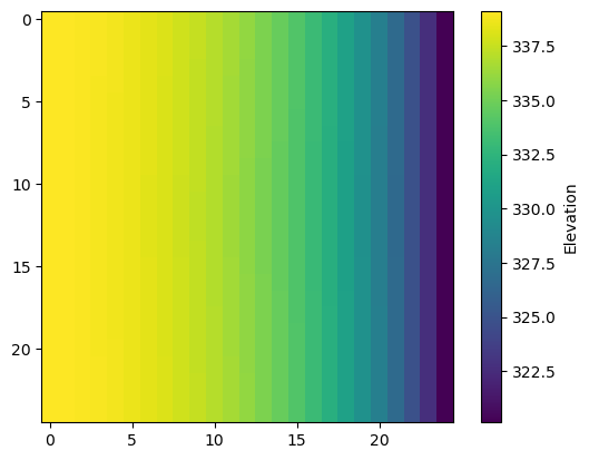
Get the water table

get_water_table() returns an nrow, ncol array of the water table elevation. This method can be useful when HDRY is turned on and the water table is in multiple layers.

[10]:

wt = get_water_table(heads=hds, hdry=-9999)

plt.imshow(wt)
plt.colorbar(label="Elevation")

[10]:

<matplotlib.colorbar.Colorbar at 0x7f2eaddd13d0>

../_images/Notebooks_modflow_postprocessing_example_16_1.png

Get layer transmissivities at arbitrary locations, accounting for the position of the water table

for this method, the heads input is an nlay x nobs array of head results, which could be constructed using the Hydmod package with an observation in each layer at each observation location, for example .
x, y values in real-world coordinates can be used in lieu of row, column, provided a correct coordinate information is supplied to the flopy model object’s grid.
open interval tops and bottoms can be supplied at each location for computing transmissivity-weighted average heads
this method can also be used for apportioning boundary fluxes for an inset from a 2-D regional model
see **flopy3_get_transmissivities_example.ipynb** for more details on how this method works

[11]:

r = [20, 5]
c = [5, 20]
headresults = hds[:, r, c]
get_transmissivities(headresults, m, r=r, c=c)

[11]:

array([[3.42867432e+03, 2.91529083e+03],
       [2.50000000e+03, 2.50000000e+03],
       [1.99999996e-01, 1.99999996e-01],
       [2.00000000e+04, 2.00000000e+04],
       [2.00000000e+04, 2.00000000e+04]])

[12]:

r = [20, 5]
c = [5, 20]
sctop = [340, 320]  # top of open interval at each location
scbot = [210, 150]  # top of bottom interval at each location
headresults = hds[:, r, c]
tr = get_transmissivities(headresults, m, r=r, c=c, sctop=sctop, scbot=scbot)
tr

[12]:

array([[3.42867432e+03, 2.50000000e+03],
       [2.50000000e+03, 2.50000000e+03],
       [9.99999978e-02, 1.99999996e-01],
       [0.00000000e+00, 1.00000000e+04],
       [0.00000000e+00, 0.00000000e+00]])

convert to transmissivity fractions

[13]:

trfrac = tr / tr.sum(axis=0)
trfrac

[13]:

array([[5.78310817e-01, 1.66664444e-01],
       [4.21672316e-01, 1.66664444e-01],
       [1.68668923e-05, 1.33331553e-05],
       [0.00000000e+00, 6.66657778e-01],
       [0.00000000e+00, 0.00000000e+00]])

Layer 3 contributes almost no transmissivity because of its K-value

[14]:

m.lpf.hk.array[:, r, c]

[14]:

array([[5.e+01, 5.e+01],
       [5.e+01, 5.e+01],
       [1.e-02, 1.e-02],
       [2.e+02, 2.e+02],
       [2.e+02, 2.e+02]], dtype=float32)

[15]:

m.modelgrid.cell_thickness[:, r, c]

[15]:

array([[130., 130.],
       [ 50.,  50.],
       [ 20.,  20.],
       [100., 100.],
       [100., 100.]])

[16]:

try:
    # ignore PermissionError on Windows
    temp_dir.cleanup()
except:
    pass