SWI2 Example 3. Freshwater-seawater interface movement in a two-aquifer coastal system
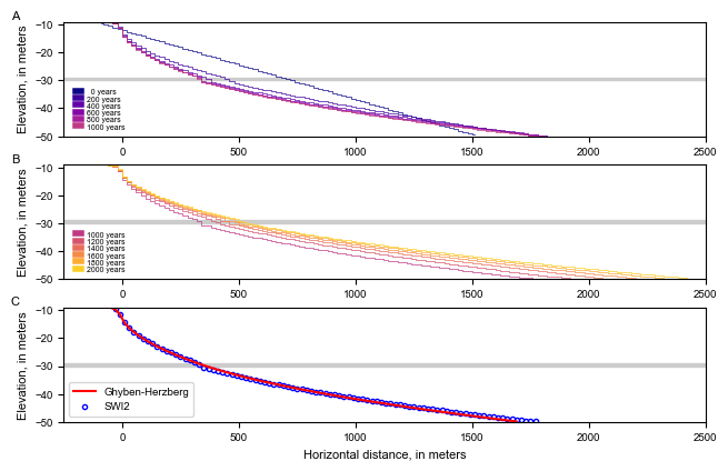
This example problem simulates transient movement of the freshwater-seawater interface in response to changing freshwater inflow in a two-aquifer coastal aquifer system. The problem domain is 4,000m long, 41m high, and 1m wide. Both aquifers are 20m thick and are separated by a leaky layer 1m thick. The aquifers are confined, storage changes are not considered (all MODFLOW stress periods are steady-state), and the top and bottom of each aquifer is horizontal. The top of the upper aquifer and bottom of the lower aquifer are impermeable.
The domain is discretized into 200 columns that are each 20m long (DELR), 1 row that is 1m wide (DELC), and 3 layers that are 20, 1, and 20m thick. A total of 2,000 years are simulated using two 1,000-year stress periods and a constant time step of 2 years. The hydraulic conductivity of the top and bottom aquifer are 2 and 4 m/d, respectively, and the horizon- tal and vertical hydraulic conductivity of the confining unit are 1 and 0.01 m/d, respectively. The effective porosity is 0.2 for all model layers.
The left 600 m of the model domain extends offshore and the ocean boundary is represented as a general head bound- ary condition (GHB) at the top of model layer 1. A freshwater head of 0 m is specified at the ocean bottom in all general head boundaries. The GHB conductance that controls outflow from the aquifer into the ocean is 0.4 square meter per day (m2/d) and corresponds to a leakance of 0.02 d-1 (or a resistance of 50 days).
The groundwater is divided into a freshwater zone and a seawater zone, separated by an active ZETA surface, ζ2, between the zones (NSRF=1) that approximates the 50-percent seawater salinity contour. Fluid density is represented using the stratified density option (ISTRAT=1). The dimensionless densities, v, of the freshwater and saltwater are 0.0 and 0.025. The tip and toe tracking parameters are a TOESLOPE of 0.02 and a TIPSLOPE of 0.04, a default ALPHA of 0.1, and a default BETA of 0.1. Initially, the interface between freshwater and seawater is straight, is at the top of aquifer 1 at x = -100, and has a slope of -0.025 m/m. The SWI2 ISOURCE parameter is set to -2 in cells having GHBs so that water that infiltrates into the aquifer from the GHB cells is saltwater (zone 2), whereas water that flows out of the model at the GHB cells is of the same type as the water at the top of the aquifer. In all other cells, the SWI2 ISOURCE parameter is set to 0, indicating boundary conditions have water that is identical to water at the top of the aquifer.
Initially, the net freshwater inflow rate of 0.03 m3/d specified at the right boundary causes flow to occur towards the ocean. The flow in each layer is distributed in proportion to the aquifer transmissivities. During the first 1,000-year stress period, a freshwater source of 0.01 m3/d is specified in the right-most cell (column 200) of the top aquifer, and a freshwater source of 0.02 m3/d is specified in the right-most cell (column 200) of the bottom aquifer. During the second 1,000-year stress period, these values are halved to reduce the net freshwater inflow to 0.015 m3/d, which is distributed in proportion to the transmissivities of both aquifers at the right boundary.
Import dependencies.
[1]:
import os
import sys
from tempfile import TemporaryDirectory

import matplotlib as mpl
import matplotlib.pyplot as plt
import numpy as np

import flopy

print(sys.version)
print(f"numpy version: {np.__version__}")
print(f"matplotlib version: {mpl.__version__}")
print(f"flopy version: {flopy.__version__}")
3.10.18 | packaged by conda-forge | (main, Jun  4 2025, 14:45:41) [GCC 13.3.0]
numpy version: 2.2.6
matplotlib version: 3.10.6
flopy version: 3.11.0.dev0
[2]:
# Modify default matplotlib settings
updates = {
    "font.family": ["Arial"],
    "mathtext.default": "regular",
    "pdf.compression": 0,
    "pdf.fonttype": 42,
    "legend.fontsize": 7,
    "axes.labelsize": 8,
    "xtick.labelsize": 7,
    "ytick.labelsize": 7,
}
plt.rcParams.update(updates)
Define some utility functions.
[3]:
def MergeData(ndim, zdata, tb):
    sv = 0.05
    md = np.empty((ndim), float)
    md.fill(np.nan)
    found = np.empty((ndim), bool)
    found.fill(False)
    for idx, layer in enumerate(zdata):
        for jdx, z in enumerate(layer):
            if found[jdx] is True:
                continue
            t0 = tb[idx][0] - sv
            t1 = tb[idx][1] + sv
            if z < t0 and z > t1:
                md[jdx] = z
                found[jdx] = True
    return md
[4]:
def LegBar(ax, x0, y0, t0, dx, dy, dt, cc):
    for c in cc:
        ax.plot([x0, x0 + dx], [y0, y0], color=c, linewidth=4)
        ctxt = f"{t0:=3d} years"
        ax.text(x0 + 2.0 * dx, y0 + dy / 2.0, ctxt, size=5)
        y0 += dy
        t0 += dt
Define model name and the location of the MODFLOW executable (assumed available on the path).
[5]:
modelname = "swiex3"
exe_name = "mf2005"
Create a temporary workspace.
[6]:
temp_dir = TemporaryDirectory()
workspace = temp_dir.name
Define model discretization.
[7]:
nlay = 3
nrow = 1
ncol = 200
delr = 20.0
delc = 1.0
Define well data.
[8]:
lrcQ1 = np.array([(0, 0, 199, 0.01), (2, 0, 199, 0.02)])
lrcQ2 = np.array([(0, 0, 199, 0.01 * 0.5), (2, 0, 199, 0.02 * 0.5)])
Define general head boundary data.
[9]:
lrchc = np.zeros((30, 5))
lrchc[:, [0, 1, 3, 4]] = [0, 0, 0.0, 0.8 / 2.0]
lrchc[:, 2] = np.arange(0, 30)
Define SWI2 data.
[10]:
zini = np.hstack((-9 * np.ones(24), np.arange(-9, -50, -0.5), -50 * np.ones(94)))[
    np.newaxis, :
]
iso = np.zeros((1, 200), dtype=int)
iso[:, :30] = -2
Create the flow model.
[11]:
ml = flopy.modflow.Modflow(
    modelname, version="mf2005", exe_name=exe_name, model_ws=workspace
)
discret = flopy.modflow.ModflowDis(
    ml,
    nrow=nrow,
    ncol=ncol,
    nlay=3,
    delr=delr,
    delc=delc,
    laycbd=[0, 0, 0],
    top=-9.0,
    botm=[-29, -30, -50],
    nper=2,
    perlen=[365 * 1000, 1000 * 365],
    nstp=[500, 500],
)
bas = flopy.modflow.ModflowBas(ml, ibound=1, strt=1.0)
bcf = flopy.modflow.ModflowBcf(
    ml, laycon=[0, 0, 0], tran=[40.0, 1, 80.0], vcont=[0.005, 0.005]
)
wel = flopy.modflow.ModflowWel(ml, stress_period_data={0: lrcQ1, 1: lrcQ2})
ghb = flopy.modflow.ModflowGhb(ml, stress_period_data={0: lrchc})
swi = flopy.modflow.ModflowSwi2(
    ml,
    iswizt=55,
    nsrf=1,
    istrat=1,
    toeslope=0.01,
    tipslope=0.04,
    nu=[0, 0.025],
    zeta=[zini, zini, zini],
    ssz=0.2,
    isource=iso,
    nsolver=1,
)
oc = flopy.modflow.ModflowOc(ml, save_every=100, save_types=["save head"])
pcg = flopy.modflow.ModflowPcg(ml)
Write the model input files.
[12]:
ml.write_input()
Run the model.
[13]:
success, buff = ml.run_model(silent=True, report=True)
assert success, "Failed to run."
Load results.
[14]:
headfile = os.path.join(workspace, f"{modelname}.hds")
hdobj = flopy.utils.HeadFile(headfile)
head = hdobj.get_data(totim=3.65000e05)
[15]:
zetafile = os.path.join(workspace, f"{modelname}.zta")
zobj = flopy.utils.CellBudgetFile(zetafile)
zkstpkper = zobj.get_kstpkper()
zeta = []
for kk in zkstpkper:
    zeta.append(zobj.get_data(kstpkper=kk, text="ZETASRF  1")[0])
zeta = np.array(zeta)
[16]:
fwid, fhgt = 7.00, 4.50
flft, frgt, fbot, ftop = 0.125, 0.95, 0.125, 0.925
Plot results.
[17]:
colormap = plt.cm.plasma  # winter
cc = []
icolor = 11
cr = np.linspace(0.0, 0.9, icolor)
for idx in cr:
    cc.append(colormap(idx))
lw = 0.5

x = np.arange(-30 * delr + 0.5 * delr, (ncol - 30) * delr, delr)
xedge = np.linspace(-30.0 * delr, (ncol - 30.0) * delr, len(x) + 1)
zedge = [[-9.0, -29.0], [-29.0, -30.0], [-30.0, -50.0]]

fig = plt.figure(figsize=(fwid, fhgt), facecolor="w")
fig.subplots_adjust(
    wspace=0.25, hspace=0.25, left=flft, right=frgt, bottom=fbot, top=ftop
)

ax = fig.add_subplot(311)
ax.text(-0.075, 1.05, "A", transform=ax.transAxes, va="center", ha="center", size="8")
# confining unit
ax.fill(
    [-600, 3400, 3400, -600],
    [-29, -29, -30, -30],
    fc=[0.8, 0.8, 0.8],
    ec=[0.8, 0.8, 0.8],
)

z = np.copy(zini[0, :])
zr = z.copy()
p = (zr < -9.0) & (zr > -50.0)
ax.plot(x[p], zr[p], color=cc[0], linewidth=lw, drawstyle="steps-mid")

for i in range(5):
    zt = MergeData(ncol, [zeta[i, 0, 0, :], zeta[i, 1, 0, :], zeta[i, 2, 0, :]], zedge)
    dr = zt.copy()
    ax.plot(x, dr, color=cc[i + 1], linewidth=lw, drawstyle="steps-mid")
# Manufacture a legend bar
LegBar(ax, -200.0, -33.75, 0, 25, -2.5, 200, cc[0:6])
# axes
ax.set_ylim(-50, -9)
ax.set_ylabel("Elevation, in meters")
ax.set_xlim(-250.0, 2500.0)

ax = fig.add_subplot(312)
ax.text(-0.075, 1.05, "B", transform=ax.transAxes, va="center", ha="center", size="8")
# confining unit
ax.fill(
    [-600, 3400, 3400, -600],
    [-29, -29, -30, -30],
    fc=[0.8, 0.8, 0.8],
    ec=[0.8, 0.8, 0.8],
)

for i in range(4, 10):
    zt = MergeData(ncol, [zeta[i, 0, 0, :], zeta[i, 1, 0, :], zeta[i, 2, 0, :]], zedge)
    dr = zt.copy()
    ax.plot(x, dr, color=cc[i + 1], linewidth=lw, drawstyle="steps-mid")
# Manufacture a legend bar
LegBar(ax, -200.0, -33.75, 1000, 25, -2.5, 200, cc[5:11])
# axes
ax.set_ylim(-50, -9)
ax.set_ylabel("Elevation, in meters")
ax.set_xlim(-250.0, 2500.0)

ax = fig.add_subplot(313)
ax.text(-0.075, 1.05, "C", transform=ax.transAxes, va="center", ha="center", size="8")
# confining unit
ax.fill(
    [-600, 3400, 3400, -600],
    [-29, -29, -30, -30],
    fc=[0.8, 0.8, 0.8],
    ec=[0.8, 0.8, 0.8],
)

zt = MergeData(ncol, [zeta[4, 0, 0, :], zeta[4, 1, 0, :], zeta[4, 2, 0, :]], zedge)
ax.plot(
    x,
    zt,
    marker="o",
    markersize=3,
    linewidth=0.0,
    markeredgecolor="blue",
    markerfacecolor="None",
)
# ghyben herzberg
zeta1 = -9 - 40.0 * (head[0, 0, :])
gbh = np.empty(len(zeta1), float)
gbho = np.empty(len(zeta1), float)
for idx, z1 in enumerate(zeta1):
    if z1 >= -9.0 or z1 <= -50.0:
        gbh[idx] = np.nan
        gbho[idx] = 0.0
    else:
        gbh[idx] = z1
        gbho[idx] = z1
ax.plot(x, gbh, "r")
np.savetxt(os.path.join(workspace, "Ghyben-Herzberg.out"), gbho)
# fake figures
ax.plot([-100.0, -100], [-100.0, -100], "r", label="Ghyben-Herzberg")
ax.plot(
    [-100.0, -100],
    [-100.0, -100],
    "bo",
    markersize=3,
    markeredgecolor="blue",
    markerfacecolor="None",
    label="SWI2",
)
# legend
leg = ax.legend(loc="lower left", numpoints=1)
leg._drawFrame = False
# axes
ax.set_ylim(-50, -9)
ax.set_xlabel("Horizontal distance, in meters")
ax.set_ylabel("Elevation, in meters")
ax.set_xlim(-250.0, 2500.0)
[17]:
(-250.0, 2500.0)
Clean up the temporary workspace.
[18]:
try:
    temp_dir.cleanup()
except (PermissionError, NotADirectoryError):
    pass