SWI2 Example 5. Radial Upconing Problem
This example problem simulates transient movement of the freshwater-seawater interface in response to groundwater withdrawals and is based on the problem of Zhou and others (2005). The aquifer is 120-m thick, confined, storage changes are not considered (because all MODFLOW stress periods are steady-state), and the top and bottom of the aquifer are horizontal and impermeable.
The domain is discretized into a radial flow domain, centered on a pumping well, having 113 columns, 1 row, and 6 layers, with respective cell dimensions of 25m (DELR), 1m (DELC), and 20m. A total of 8 years is simulated using two 4-year stress periods and a constant 1-day time step.
The horizontal and vertical hydraulic conductivity of the aquifer are 21.7 and 8.5 m/d, respectively, and the effective porosity of the aquifer is 0.2. The hydraulic conductivity and effective porosity values applied in the model are based on the approach of logarithmic averaging of interblock transmissivity (LAYAVG=1) to better approximate analytical solutions for radial flow problems (Langevin, 2008). Constant heads were specified at the edge of the model domain (column 113) in all 6 layers, with specified freshwater heads of 0.0m.
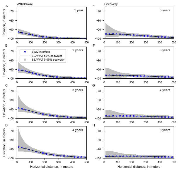
The groundwater is divided into a freshwater zone and a seawater zone, separated by an active ZETA surface, ζ2, between the zones (NSRF=1) that approximates the 50-percent seawater salinity contour. Fluid density is represented using the stratified density option (ISTRAT=1). The dimensionless density difference between freshwater and saltwater is 0.025. The tip and toe tracking parameters are a TOESLOPE and TIPSLOPE of 0.025, a default ALPHA of 0.1, and a default BETA of 0.1. Initially, the interface between freshwater and saltwater is at an elevation of -100m. The SWI2 ISOURCE parameter is set to 1 in the constant head cells in layers 1-5 and to 2 in the constant head cell in layer 6. This ensures that inflow from the constant head cells in model layers 1-5 and 6 is freshwater and saltwater, respectively. In all other cells, the SWI2 ISOURCE parameter was set to 0, indicating boundary conditions have water that is identical to water at the top of the aquifer.
A pumping well screened from 0 to -20m with a withdrawal rate of 2,400 m3/d is simulated for stress period 1 at the left side of the model (column 1) in the first layer. To simulate recovery, the pumping well withdrawal rate was set to 0 m3/d for stress period 2.
The simulated position of the interface is shown at 1-year increments for the withdrawal (stress period 1) and recovery (stress period 2) periods. During the withdrawal period, the interface steadily rises from its initial elevation of -100m to a maximum elevation of -87m after 4 years. During the recovery period, the interface elevation decreases to -96m at the end of year 5 but does not return to the initial elevation of -100m at the end of year 8.
Import dependencies.
[1]:
import math
import os
import sys
from tempfile import TemporaryDirectory

import matplotlib as mpl
import matplotlib.pyplot as plt
import numpy as np

import flopy

print(sys.version)
print(f"numpy version: {np.__version__}")
print(f"matplotlib version: {mpl.__version__}")
print(f"flopy version: {flopy.__version__}")
3.10.18 | packaged by conda-forge | (main, Jun  4 2025, 14:45:41) [GCC 13.3.0]
numpy version: 2.2.6
matplotlib version: 3.10.6
flopy version: 3.11.0.dev0
[2]:
# Modify default matplotlib settings.
updates = {
    "font.family": ["Arial"],
    "mathtext.default": "regular",
    "pdf.compression": 0,
    "pdf.fonttype": 42,
    "legend.fontsize": 7,
    "axes.labelsize": 8,
    "xtick.labelsize": 7,
    "ytick.labelsize": 7,
}
plt.rcParams.update(updates)
Create a temporary workspace.
[3]:
temp_dir = TemporaryDirectory()
workspace = temp_dir.name
Make working subdirectories.
[4]:
dirs = [os.path.join(workspace, "SWI2"), os.path.join(workspace, "SEAWAT")]
for d in dirs:
    if not os.path.exists(d):
        os.mkdir(d)
Define grid discretization.
[5]:
nlay = 6
nrow = 1
ncol = 113
delr = np.zeros((ncol), float)
delc = 1.0
r = np.zeros((ncol), float)
x = np.zeros((ncol), float)
edge = np.zeros((ncol), float)
dx = 25.0
for i in range(0, ncol):
    delr[i] = dx
r[0] = delr[0] / 2.0
for i in range(1, ncol):
    r[i] = r[i - 1] + (delr[i - 1] + delr[i]) / 2.0
x[0] = delr[0] / 2.0
for i in range(1, ncol):
    x[i] = x[i - 1] + (delr[i - 1] + delr[i]) / 2.0
edge[0] = delr[0]
for i in range(1, ncol):
    edge[i] = edge[i - 1] + delr[i]
Define time discretization.
[6]:
nper = 2
perlen = [1460, 1460]
nstp = [1460, 1460]
steady = True
Define more shared model parameters.
[7]:
nsave_zeta = 8
ndecay = 4
ibound = np.ones((nlay, nrow, ncol), int)
for k in range(0, nlay):
    ibound[k, 0, ncol - 1] = -1
bot = np.zeros((nlay, nrow, ncol), float)
dz = 100.0 / float(nlay - 1)
zall = -np.arange(0, 100 + dz, dz)
zall = np.append(zall, -120.0)
tb = -np.arange(dz, 100 + dz, dz)
tb = np.append(tb, -120.0)
for k in range(0, nlay):
    for i in range(0, ncol):
        bot[k, 0, i] = tb[k]
isource = np.zeros((nlay, nrow, ncol), int)
isource[:, 0, ncol - 1] = 1
isource[nlay - 1, 0, ncol - 1] = 2

khb = (0.0000000000256 * 1000.0 * 9.81 / 0.001) * 60 * 60 * 24
kvb = (0.0000000000100 * 1000.0 * 9.81 / 0.001) * 60 * 60 * 24
ssb = 1e-5
sszb = 0.2
kh = np.zeros((nlay, nrow, ncol), float)
kv = np.zeros((nlay, nrow, ncol), float)
ss = np.zeros((nlay, nrow, ncol), float)
ssz = np.zeros((nlay, nrow, ncol), float)
for k in range(0, nlay):
    for i in range(0, ncol):
        f = r[i] * 2.0 * math.pi
        kh[k, 0, i] = khb * f
        kv[k, 0, i] = kvb * f
        ss[k, 0, i] = ssb * f
        ssz[k, 0, i] = sszb * f
z = np.ones((nlay), float)
z = -100.0 * z

nwell = 1
for k in range(0, nlay):
    if zall[k] > -20.0 and zall[k + 1] <= -20:
        nwell = k + 1
print(f"nlay={nlay} dz={dz} nwell={nwell}")
wellQ = -2400.0
wellbtm = -20.0
wellQpm = wellQ / abs(wellbtm)
well_data = {}
for ip in range(0, nper):
    welllist = np.zeros((nwell, 4), float)
    for iw in range(0, nwell):
        if ip == 0:
            b = zall[iw] - zall[iw + 1]
            if zall[iw + 1] < wellbtm:
                b = zall[iw] - wellbtm
            q = wellQpm * b
        else:
            q = 0.0
        welllist[iw, 0] = iw
        welllist[iw, 1] = 0
        welllist[iw, 2] = 0
        welllist[iw, 3] = q
    well_data[ip] = welllist.copy()

ihead = np.zeros((nlay), float)

ocspd = {}
for i in range(0, nper):
    icnt = 0
    for j in range(0, nstp[i]):
        icnt += 1
        if icnt == 365:
            ocspd[i, j] = ["save head"]
            icnt = 0
        else:
            ocspd[i, j] = []

solver2params = {
    "mxiter": 100,
    "iter1": 20,
    "npcond": 1,
    "zclose": 1.0e-6,
    "rclose": 3e-3,
    "relax": 1.0,
    "nbpol": 2,
    "damp": 1.0,
    "dampt": 1.0,
}
nlay=6 dz=20.0 nwell=1
Define SWI2 model name and MODFLOW executable name.
[8]:
modelname = "swi2ex5"
mf_name = "mf2005"
Define the SWI2 model.
[9]:
ml = flopy.modflow.Modflow(
    modelname, version="mf2005", exe_name=mf_name, model_ws=dirs[0]
)
discret = flopy.modflow.ModflowDis(
    ml,
    nrow=nrow,
    ncol=ncol,
    nlay=nlay,
    delr=delr,
    delc=delc,
    top=0,
    botm=bot,
    laycbd=0,
    nper=nper,
    perlen=perlen,
    nstp=nstp,
    steady=steady,
)
bas = flopy.modflow.ModflowBas(ml, ibound=ibound, strt=ihead)
lpf = flopy.modflow.ModflowLpf(
    ml, hk=kh, vka=kv, ss=ss, sy=ssz, vkcb=0, laytyp=0, layavg=1
)
wel = flopy.modflow.ModflowWel(ml, stress_period_data=well_data)
swi = flopy.modflow.ModflowSwi2(
    ml,
    iswizt=55,
    nsrf=1,
    istrat=1,
    toeslope=0.025,
    tipslope=0.025,
    nu=[0, 0.025],
    zeta=z,
    ssz=ssz,
    isource=isource,
    nsolver=2,
    solver2params=solver2params,
)
oc = flopy.modflow.ModflowOc(ml, stress_period_data=ocspd)
pcg = flopy.modflow.ModflowPcg(ml, hclose=1.0e-6, rclose=3.0e-3, mxiter=100, iter1=50)
Write input files and run the SWI2 model.
[10]:
ml.write_input()
success, buff = ml.run_model(silent=True, report=True)
assert success, "Failed to run."
[11]:
# Load model results.
get_stp = [364, 729, 1094, 1459, 364, 729, 1094, 1459]
get_per = [0, 0, 0, 0, 1, 1, 1, 1]
nswi_times = len(get_per)
zetafile = os.path.join(dirs[0], f"{modelname}.zta")
zobj = flopy.utils.CellBudgetFile(zetafile)
zeta = []
for kk in zip(get_stp, get_per):
    zeta.append(zobj.get_data(kstpkper=kk, text="ZETASRF  1")[0])
zeta = np.array(zeta)
Redefine input data for SEAWAT.
[12]:
nlay_swt = 120
# mt3d print times
timprs = (np.arange(8) + 1) * 365.0
nprs = len(timprs)
ndecay = 4
ibound = np.ones((nlay_swt, nrow, ncol), "int")
for k in range(0, nlay_swt):
    ibound[k, 0, ncol - 1] = -1
bot = np.zeros((nlay_swt, nrow, ncol), float)
zall = [0, -20.0, -40.0, -60.0, -80.0, -100.0, -120.0]
dz = 120.0 / nlay_swt
tb = np.arange(nlay_swt) * -dz - dz
sconc = np.zeros((nlay_swt, nrow, ncol), float)
icbund = np.ones((nlay_swt, nrow, ncol), int)
strt = np.zeros((nlay_swt, nrow, ncol), float)
pressure = 0.0
g = 9.81
z = -dz / 2.0  # cell center
for k in range(0, nlay_swt):
    for i in range(0, ncol):
        bot[k, 0, i] = tb[k]
    if bot[k, 0, 0] >= -100.0:
        sconc[k, 0, :] = 0.0 / 3.0 * 0.025 * 1000.0 / 0.7143
    else:
        sconc[k, 0, :] = 3.0 / 3.0 * 0.025 * 1000.0 / 0.7143
        icbund[k, 0, -1] = -1

    dense = 1000.0 + 0.7143 * sconc[k, 0, 0]
    pressure += 0.5 * dz * dense * g
    if k > 0:
        z = z - dz
        denseup = 1000.0 + 0.7143 * sconc[k - 1, 0, 0]
        pressure += 0.5 * dz * denseup * g
    strt[k, 0, :] = z + pressure / dense / g
    # print z, pressure, strt[k, 0, 0], sconc[k, 0, 0]

khb = (0.0000000000256 * 1000.0 * 9.81 / 0.001) * 60 * 60 * 24
kvb = (0.0000000000100 * 1000.0 * 9.81 / 0.001) * 60 * 60 * 24
ssb = 1e-5
sszb = 0.2
kh = np.zeros((nlay_swt, nrow, ncol), float)
kv = np.zeros((nlay_swt, nrow, ncol), float)
ss = np.zeros((nlay_swt, nrow, ncol), float)
ssz = np.zeros((nlay_swt, nrow, ncol), float)
for k in range(0, nlay_swt):
    for i in range(0, ncol):
        f = r[i] * 2.0 * math.pi
        kh[k, 0, i] = khb * f
        kv[k, 0, i] = kvb * f
        ss[k, 0, i] = ssb * f
        ssz[k, 0, i] = sszb * f
# wells and ssm data
itype = flopy.mt3d.Mt3dSsm.itype_dict()
nwell = 1
for k in range(0, nlay_swt):
    if bot[k, 0, 0] >= -20.0:
        nwell = k + 1
print(f"nlay_swt={nlay_swt} dz={dz} nwell={nwell}")
well_data = {}
ssm_data = {}
wellQ = -2400.0
wellbtm = -20.0
wellQpm = wellQ / abs(wellbtm)
for ip in range(0, nper):
    welllist = np.zeros((nwell, 4), float)
    ssmlist = []
    for iw in range(0, nwell):
        if ip == 0:
            q = wellQpm * dz
        else:
            q = 0.0
        welllist[iw, 0] = iw
        welllist[iw, 1] = 0
        welllist[iw, 2] = 0
        welllist[iw, 3] = q
        ssmlist.append([iw, 0, 0, 0.0, itype["WEL"]])
    well_data[ip] = welllist.copy()
    ssm_data[ip] = ssmlist
nlay_swt=120 dz=1.0 nwell=20
Define model name and exe for SEAWAT model.
[13]:
modelname = "swi2ex5_swt"
swtexe_name = "swtv4"
Create the SEAWAT model.
[14]:
m = flopy.seawat.Seawat(modelname, exe_name=swtexe_name, model_ws=dirs[1])
discret = flopy.modflow.ModflowDis(
    m,
    nrow=nrow,
    ncol=ncol,
    nlay=nlay_swt,
    delr=delr,
    delc=delc,
    top=0,
    botm=bot,
    laycbd=0,
    nper=nper,
    perlen=perlen,
    nstp=nstp,
    steady=True,
)
bas = flopy.modflow.ModflowBas(m, ibound=ibound, strt=strt)
lpf = flopy.modflow.ModflowLpf(
    m, hk=kh, vka=kv, ss=ss, sy=ssz, vkcb=0, laytyp=0, layavg=1
)
wel = flopy.modflow.ModflowWel(m, stress_period_data=well_data)
oc = flopy.modflow.ModflowOc(m, save_every=365, save_types=["save head"])
pcg = flopy.modflow.ModflowPcg(m, hclose=1.0e-5, rclose=3.0e-3, mxiter=100, iter1=50)
# Create the basic MT3DMS model data
adv = flopy.mt3d.Mt3dAdv(
    m,
    mixelm=-1,
    percel=0.5,
    nadvfd=0,
    # 0 or 1 is upstream; 2 is central in space
    # particle based methods
    nplane=4,
    mxpart=1e7,
    itrack=2,
    dceps=1e-4,
    npl=16,
    nph=16,
    npmin=8,
    npmax=256,
)
btn = flopy.mt3d.Mt3dBtn(
    m,
    icbund=icbund,
    prsity=ssz,
    ncomp=1,
    sconc=sconc,
    ifmtcn=-1,
    chkmas=False,
    nprobs=10,
    nprmas=10,
    dt0=1.0,
    ttsmult=1.0,
    nprs=nprs,
    timprs=timprs,
    mxstrn=1e8,
)
dsp = flopy.mt3d.Mt3dDsp(m, al=0.0, trpt=1.0, trpv=1.0, dmcoef=0.0)
gcg = flopy.mt3d.Mt3dGcg(m, mxiter=1, iter1=50, isolve=1, cclose=1e-7)
ssm = flopy.mt3d.Mt3dSsm(m, stress_period_data=ssm_data)
# Create the SEAWAT model data
vdf = flopy.seawat.SeawatVdf(
    m,
    iwtable=0,
    densemin=0,
    densemax=0,
    denseref=1000.0,
    denseslp=0.7143,
    firstdt=1e-3,
)
Write SEAWAT model input files.
[15]:
m.write_input()
Run the SEAWAT model.
[16]:
success, buff = m.run_model(silent=True, report=True)
assert success, "Failed to run."
Load SEAWAT model results.
[17]:
ucnfile = os.path.join(dirs[1], "MT3D001.UCN")
uobj = flopy.utils.UcnFile(ucnfile)
times = uobj.get_times()
print(times)
conc = np.zeros((len(times), nlay_swt, ncol), float)
for idx, tt in enumerate(times):
    c = uobj.get_data(totim=tt)
    for ilay in range(0, nlay_swt):
        for jcol in range(0, ncol):
            conc[idx, ilay, jcol] = c[ilay, 0, jcol]
[np.float32(365.0), np.float32(730.0), np.float32(1095.0), np.float32(1460.0), np.float32(1825.0), np.float32(2190.0), np.float32(2555.0), np.float32(2920.0)]
Define some spatial data for plots.
[18]:
# swi2
bot = np.zeros((1, ncol, nlay), float)
dz = 100.0 / float(nlay - 1)
zall = -np.arange(0, 100 + dz, dz)
zall = np.append(zall, -120.0)
tb = -np.arange(dz, 100 + dz, dz)
tb = np.append(tb, -120.0)
for k in range(0, nlay):
    for i in range(0, ncol):
        bot[0, i, k] = tb[k]
# seawat
swt_dz = 120.0 / nlay_swt
swt_tb = np.zeros((nlay_swt), float)
zc = -swt_dz / 2.0
for klay in range(0, nlay_swt):
    swt_tb[klay] = zc
    zc -= swt_dz
X, Z = np.meshgrid(x, swt_tb)
Plot results.
[19]:
fwid, fhgt = 6.5, 6.5
flft, frgt, fbot, ftop = 0.125, 0.95, 0.125, 0.925

eps = 1.0e-3

lc = ["r", "c", "g", "b", "k"]
cfig = ["A", "B", "C", "D", "E", "F", "G", "H"]
inc = 1.0e-3

xsf, axes = plt.subplots(4, 2, figsize=(fwid, fhgt), facecolor="w")
xsf.subplots_adjust(
    wspace=0.25, hspace=0.25, left=flft, right=frgt, bottom=fbot, top=ftop
)
# withdrawal and recovery titles
ax = axes.flatten()[0]
ax.text(
    0.0, 1.03, "Withdrawal", transform=ax.transAxes, va="bottom", ha="left", size="8"
)
ax = axes.flatten()[1]
ax.text(0.0, 1.03, "Recovery", transform=ax.transAxes, va="bottom", ha="left", size="8")
# dummy items for legend
ax = axes.flatten()[2]
ax.plot(
    [-1, -1],
    [-1, -1],
    "bo",
    markersize=3,
    markeredgecolor="blue",
    markerfacecolor="None",
    label="SWI2 interface",
)
ax.plot(
    [-1, -1],
    [-1, -1],
    color="k",
    linewidth=0.75,
    linestyle="solid",
    label="SEAWAT 50% seawater",
)
ax.plot(
    [-1, -1],
    [-1, -1],
    marker="s",
    color="k",
    linewidth=0,
    linestyle="none",
    markeredgecolor="w",
    markerfacecolor="0.75",
    label="SEAWAT 5-95% seawater",
)
leg = ax.legend(
    loc="upper left",
    numpoints=1,
    ncol=1,
    labelspacing=0.5,
    borderaxespad=1,
    handlelength=3,
)
leg._drawFrame = False
# data items
for itime in range(0, nswi_times):
    zb = np.zeros((ncol), float)
    zs = np.zeros((ncol), float)
    for icol in range(0, ncol):
        for klay in range(0, nlay):
            # top and bottom of layer
            ztop = float(f"{zall[klay]:10.3e}")
            zbot = float(f"{zall[klay + 1]:10.3e}")
            # fresh-salt zeta surface
            zt = zeta[itime, klay, 0, icol]
            if (ztop - zt) > eps:
                zs[icol] = zt
    if itime < ndecay:
        ic = itime
        isp = ic * 2
        ax = axes.flatten()[isp]
    else:
        ic = itime - ndecay
        isp = (ic * 2) + 1
        ax = axes.flatten()[isp]
    # figure title
    ax.text(
        -0.15,
        1.025,
        cfig[itime],
        transform=ax.transAxes,
        va="center",
        ha="center",
        size="8",
    )

    # swi2
    ax.plot(
        x,
        zs,
        "bo",
        markersize=3,
        markeredgecolor="blue",
        markerfacecolor="None",
        label="_None",
    )

    # seawat
    sc = ax.contour(
        X,
        Z,
        conc[itime, :, :],
        levels=[17.5],
        colors="k",
        linestyles="solid",
        linewidths=0.75,
        zorder=30,
    )
    cc = ax.contourf(
        X, Z, conc[itime, :, :], levels=[0.0, 1.75, 33.250], colors=["w", "0.75", "w"]
    )
    # set graph limits
    ax.set_xlim(0, 500)
    ax.set_ylim(-100, -65)
    if itime < ndecay:
        ax.set_ylabel("Elevation, in meters")

# x labels
ax = axes.flatten()[6]
ax.set_xlabel("Horizontal distance, in meters")
ax = axes.flatten()[7]
ax.set_xlabel("Horizontal distance, in meters")

# simulation time titles
for itime in range(0, nswi_times):
    if itime < ndecay:
        ic = itime
        isp = ic * 2
        ax = axes.flatten()[isp]
    else:
        ic = itime - ndecay
        isp = (ic * 2) + 1
        ax = axes.flatten()[isp]
    iyr = itime + 1
    if iyr > 1:
        ctxt = f"{iyr} years"
    else:
        ctxt = f"{iyr} year"
    ax.text(0.95, 0.925, ctxt, transform=ax.transAxes, va="top", ha="right", size="8")

plt.show()
Clean up the temporary workspace.
[20]:
try:
    temp_dir.cleanup()
except (PermissionError, NotADirectoryError):
    pass